
The R package FFTrees creates, visualizes and evaluates fast-and-frugal decision trees (FFTs) for solving binary classification tasks following the methods described in Phillips, Neth, Woike & Gaissmaier (2017, as html | PDF).
Fast-and-frugal trees (FFTs) are simple and transparent decision algorithms for solving binary classification problems. The key feature making FFTs faster and more frugal than other decision trees is that every node allows for a decision. When predicting new outcomes, the performance of FFTs competes with more complex algorithms and machine learning techniques, such as logistic regression (LR), support-vector machines (SVM), and random forests (RF). Apart from being faster and requiring less information, FFTs tend to be robust against overfitting, and easy to interpret, use, and communicate.
To install the latest release of FFTrees from CRAN evaluate:
install.packages("FFTrees")The current development version of FFTrees can be installed from GitHub with:
# install.packages("devtools")
devtools::install_github("ndphillips/FFTrees", build_vignettes = TRUE)As an example, let’s create a FFT predicting heart disease status
(Healthy vs. Diseased) based on the
heartdisease dataset included in
FFTrees:
library(FFTrees) # load packageThe heartdisease data provides medical information for
303 patients that were tested for heart disease. The full data were
split into two subsets: A heart.train dataset for fitting
decision trees, and heart.test dataset for a testing the
resulting trees. Here are the first rows and columns of both subsets of
the heartdisease data:
heart.train (the training / fitting dataset) contains
the data from 150 patients:heart.train
#> # A tibble: 150 × 14
#> diagnosis age sex cp trestbps chol fbs restecg thalach exang
#> <lgl> <dbl> <dbl> <chr> <dbl> <dbl> <dbl> <chr> <dbl> <dbl>
#> 1 FALSE 44 0 np 108 141 0 normal 175 0
#> 2 FALSE 51 0 np 140 308 0 hypertrophy 142 0
#> 3 FALSE 52 1 np 138 223 0 normal 169 0
#> 4 TRUE 48 1 aa 110 229 0 normal 168 0
#> 5 FALSE 59 1 aa 140 221 0 normal 164 1
#> 6 FALSE 58 1 np 105 240 0 hypertrophy 154 1
#> 7 FALSE 41 0 aa 126 306 0 normal 163 0
#> 8 TRUE 39 1 a 118 219 0 normal 140 0
#> 9 TRUE 77 1 a 125 304 0 hypertrophy 162 1
#> 10 FALSE 41 0 aa 105 198 0 normal 168 0
#> # … with 140 more rows, and 4 more variables: oldpeak <dbl>, slope <chr>,
#> # ca <dbl>, thal <chr>heart.test (the testing / prediction dataset) contains
data from a new set of 153 patients:heart.test
#> # A tibble: 153 × 14
#> diagnosis age sex cp trestbps chol fbs restecg thalach exang
#> <lgl> <dbl> <dbl> <chr> <dbl> <dbl> <dbl> <chr> <dbl> <dbl>
#> 1 FALSE 51 0 np 120 295 0 hypertrophy 157 0
#> 2 TRUE 45 1 ta 110 264 0 normal 132 0
#> 3 TRUE 53 1 a 123 282 0 normal 95 1
#> 4 TRUE 45 1 a 142 309 0 hypertrophy 147 1
#> 5 FALSE 66 1 a 120 302 0 hypertrophy 151 0
#> 6 TRUE 48 1 a 130 256 1 hypertrophy 150 1
#> 7 TRUE 55 1 a 140 217 0 normal 111 1
#> 8 FALSE 56 1 aa 130 221 0 hypertrophy 163 0
#> 9 TRUE 42 1 a 136 315 0 normal 125 1
#> 10 FALSE 45 1 a 115 260 0 hypertrophy 185 0
#> # … with 143 more rows, and 4 more variables: oldpeak <dbl>, slope <chr>,
#> # ca <dbl>, thal <chr>Most of the variables in our data are potential predictors. The
criterion variable is diagnosis — a logical column
indicating the true state for each patient (TRUE
or FALSE, i.e., whether or not the patient suffers from
heart disease).
Now let’s use FFTrees() to create FFTs for the
heart.train data and evaluate their predictive performance
on the heart.test data:
FFTrees object from the
heartdisease data:# Create an FFTrees object from the heartdisease data:
heart.fft <- FFTrees(formula = diagnosis ~.,
data = heart.train,
data.test = heart.test,
decision.labels = c("Healthy", "Disease"))
#> Setting 'goal = bacc'
#> Setting 'goal.chase = bacc'
#> Setting 'goal.threshold = bacc'
#> Setting cost.outcomes = list(hi = 0, mi = 1, fa = 1, cr = 0)
#> Growing FFTs with ifan:
#> Fitting other algorithms for comparison (disable with do.comp = FALSE) ...FFTrees object shows basic information and
summary statistics (on the best training tree, FFT #1):# Print:
heart.fft
#> FFTrees
#> - Trees: 7 fast-and-frugal trees predicting diagnosis
#> - Outcome costs: [hi = 0, mi = 1, fa = 1, cr = 0]
#>
#> FFT #1: Definition
#> [1] If thal = {rd,fd}, decide Disease.
#> [2] If cp != {a}, decide Healthy.
#> [3] If ca > 0, decide Disease, otherwise, decide Healthy.
#>
#> FFT #1: Training Accuracy
#> Training data: N = 150, Pos (+) = 66 (44%)
#>
#> | | True + | True - | Totals:
#> |----------|--------|--------|
#> | Decide + | hi 54 | fa 18 | 72
#> | Decide - | mi 12 | cr 66 | 78
#> |----------|--------|--------|
#> Totals: 66 84 N = 150
#>
#> acc = 80.0% ppv = 75.0% npv = 84.6%
#> bacc = 80.2% sens = 81.8% spec = 78.6%
#>
#> FFT #1: Training Speed, Frugality, and Cost
#> mcu = 1.74, pci = 0.87, E(cost) = 0.200FFTrees object to visualize a tree and its performance (on
the test data):# Plot the best tree applied to the test data:
plot(heart.fft,
data = "test",
main = "Heart Disease")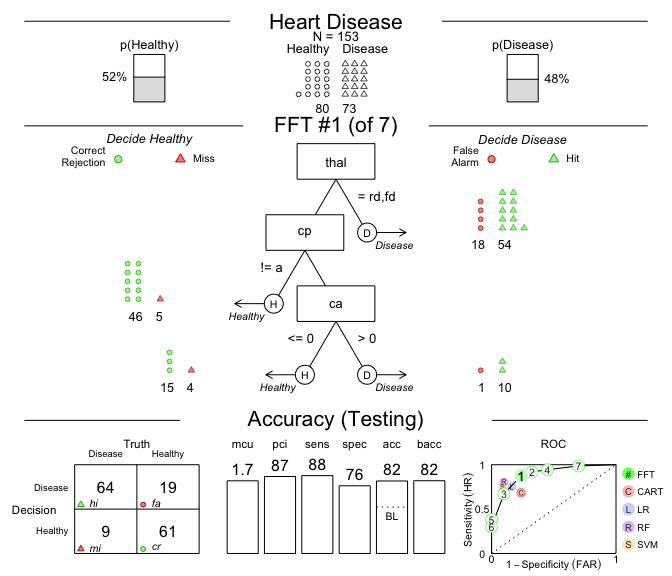
Figure 1: A fast-and-frugal tree (FFT) predicting
heart disease for test data and its performance
characteristics.
# Compare predictive performance across algorithms:
heart.fft$competition$test
#> # A tibble: 5 × 16
#>   algorithm     n    hi    fa    mi    cr  sens  spec    far   ppv   npv   acc
#>   <chr>     <int> <int> <int> <int> <int> <dbl> <dbl>  <dbl> <dbl> <dbl> <dbl>
#> 1 fftrees     153    64    19     9    61 0.877 0.762 0.238  0.771 0.871 0.817
#> 2 lr          153    55    13    18    67 0.753 0.838 0.162  0.809 0.788 0.797
#> 3 cart        153    50    19    23    61 0.685 0.762 0.238  0.725 0.726 0.725
#> 4 rf          153    59     8    14    72 0.808 0.9   0.1    0.881 0.837 0.856
#> 5 svm         153    55     7    18    73 0.753 0.912 0.0875 0.887 0.802 0.837
#> # … with 4 more variables: bacc <dbl>, cost <dbl>, cost_decisions <dbl>,
#> # cost_cues <dbl>Because fast-and-frugal trees are so simple, we even can create FFTs ‘from words’ and apply them to data!
For example, let’s create a tree with the following three nodes and
evaluate its performance on the heart.test data:
sex = 1, predict Disease.age < 45, predict Healthy.thal = {fd, normal}, predict Healthy,These conditions can directly be supplied to the my.tree
argument of FFTrees():
# Create custom FFT 'in words' and apply it to test data:

# 1. Create my own FFT (from verbal description):
my.fft <- FFTrees(formula = diagnosis ~.,
                  data = heart.train,
                  data.test = heart.test,
                  decision.labels = c("Healthy", "Disease"),
                  my.tree = "If sex = 1, predict Disease.
                             If age < 45, predict Healthy.
                             If thal = {fd, normal}, predict Healthy,
                             Otherwise, predict Disease.")

# 2. Plot and evaluate my custom FFT (for test data):
plot(my.fft,
     data = "test",
     main = "My custom FFT")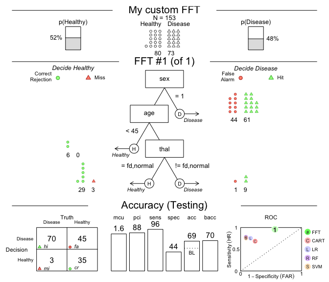
Figure 2: An FFT predicting heart disease created from a verbal description.
As we can see, this particular tree is somewhat biased: It has nearly perfect sensitivity (i.e., is good at identifying cases of Disease) but suffers from low specificity (i.e., is not so good at identifying Healthy cases). Overall, the accuracy of our custom tree exceeds the data’s baseline by a fair amount. However, exploring FFTrees further will quickly enable you to design much better FFTs.
We had a lot of fun creating FFTrees and hope you like it too! As a comprehensive, yet accessible introduction to FFTs, we recommend reading our article in the journal Judgment and Decision Making (2017, volume 12, issue 4), entitled FFTrees: A toolbox to create, visualize,and evaluate fast-and-frugal decision trees (available in html | PDF ).
Citation (in APA format):
We encourage you to read the article to learn more about the history of FFTs and how the FFTrees package creates, visualizes, and evaluates them. If you use FFTrees in your own work, please cite us and share your experiences (e.g., on GitHub) so we can continue developing the package.
Here are some scientific publications that have used FFTrees (see Google Scholar for the full list):
[File README.Rmd last updated on 2022-08-31.]