
HotellingEllipse computes the lengths of the semi-minor
and semi-major axes for plotting Hotelling ellipse at 95% and 99%
confidence intervals. The package also provides the
x-y coordinates at user-defined confidence
intervals.
Install HotellingEllipse from CRAN:
install.packages("HotellingEllipse")Install the development version from GitHub:
# install.packages("remotes")
remotes::install_github("ChristianGoueguel/HotellingEllipse")Below is an overview of how HotellingEllipse can help
draw a confidence ellipse:
using FactoMineR::PCA() we first perform Principal
Component Analysis (PCA) from a LIBS spectral dataset
data("specData") and extract the PCA scores.
with ellipseParam() we get the Hotelling’s T-squared
statistic along with the values of the semi-minor and semi-major axes.
Whereas, ellipseCoord() provides the x and
y coordinates for drawing the Hotelling ellipse at user-defined
confidence interval.
using ggplot2::ggplot() and
ggforce::geom_ellipse() we plot the scatterplot of PCA
scores as well as the corresponding Hotelling ellipse which represents
the confidence region for the joint variables at 99% and 95% confidence
intervals.
Step 1. Load the package.
library(HotellingEllipse)Step 2. Load LIBS dataset.
data("specData")Step 3. Perform principal component analysis.
set.seed(123)
pca_mod <- specData %>%
  select(where(is.numeric)) %>%
  PCA(scale.unit = FALSE, graph = FALSE)
Step 4. Extract PCA scores.
pca_scores <- pca_mod %>%
  pluck("ind", "coord") %>%
  as_tibble() %>%
  print()
#> # A tibble: 100 × 5
#>      Dim.1   Dim.2  Dim.3  Dim.4   Dim.5
#>      <dbl>   <dbl>  <dbl>  <dbl>   <dbl>
#>  1  17689. -20927.  2599. -1570. -3691.
#>  2   -775.   -806. -2700. -3263.   989.
#>  3  -2401.   -273. -1839. -2279.  -324.
#>  4   2862.   6557.  1465.  4453.   -49.7
#>  5   6379.   3538. -3310.  1160.   496.
#>  6   8251.   2326.  3907. -2607. -1172.
#>  7 -13022.  -3948.  1698.  4685. -1222.
#>  8  -4671.   1999.  3042.  1516.   -75.7
#>  9  -1460.    800. -2420. -3238.   477.
#> 10  19271.  -6668.  -413.  1615.  2149.
#> # … with 90 more rows
Step 5. Run ellipseParam() for the
first two principal components (k = 2). We want to
compute the length of the semi-axes of the Hotelling ellipse (denoted
a and b) when the first principal
component, PC1, is on the x-axis (pcx = 1)
and, the second principal component, PC2, is on the y-axis
(pcy = 2).
res_2PCs <- ellipseParam(data = pca_scores, k = 2, pcx = 1, pcy = 2)str(res_2PCs)
#> List of 4
#> $ Tsquare : tibble [100 × 1] (S3: tbl_df/tbl/data.frame)
#> ..$ value: num [1:100] 13.738 1.418 0.692 2.761 1.313 ...
#> $ Ellipse : tibble [1 × 4] (S3: tbl_df/tbl/data.frame)
#> ..$ a.99pct: num 21419
#> ..$ b.99pct: num 16002
#> ..$ a.95pct: num 17132
#> ..$ b.95pct: num 12799
#> $ cutoff.99pct: num 9.76
#> $ cutoff.95pct: num 6.24a1 <- pluck(res_2PCs, "Ellipse", "a.99pct")
b1 <- pluck(res_2PCs, "Ellipse", "b.99pct")a2 <- pluck(res_2PCs, "Ellipse", "a.95pct")
b2 <- pluck(res_2PCs, "Ellipse", "b.95pct")T2 <- pluck(res_2PCs, "Tsquare", "value")Another way to add Hotelling ellipse on the scatterplot of the scores
is to use the function ellipseCoord(). This function
provides the x and y coordinates of the confidence
ellipse at user-defined confidence interval. The confidence interval
conf.limit is set at 95% by default. Here, PC1 is on the
x-axis (pcx = 1) and, the third principal
component, PC3, is on the y-axis (pcy =
3).
coord_2PCs_99 <- ellipseCoord(data = pca_scores, pcx = 1, pcy = 3, conf.limit = 0.99, pts = 500)
coord_2PCs_95 <- ellipseCoord(data = pca_scores, pcx = 1, pcy = 3, conf.limit = 0.95, pts = 500)
coord_2PCs_90 <- ellipseCoord(data = pca_scores, pcx = 1, pcy = 3, conf.limit = 0.90, pts = 500)str(coord_2PCs_99)
#> tibble [500 × 2] (S3: tbl_df/tbl/data.frame)
#> $ x: num [1:500] 21419 21418 21412 21404 21392 ...
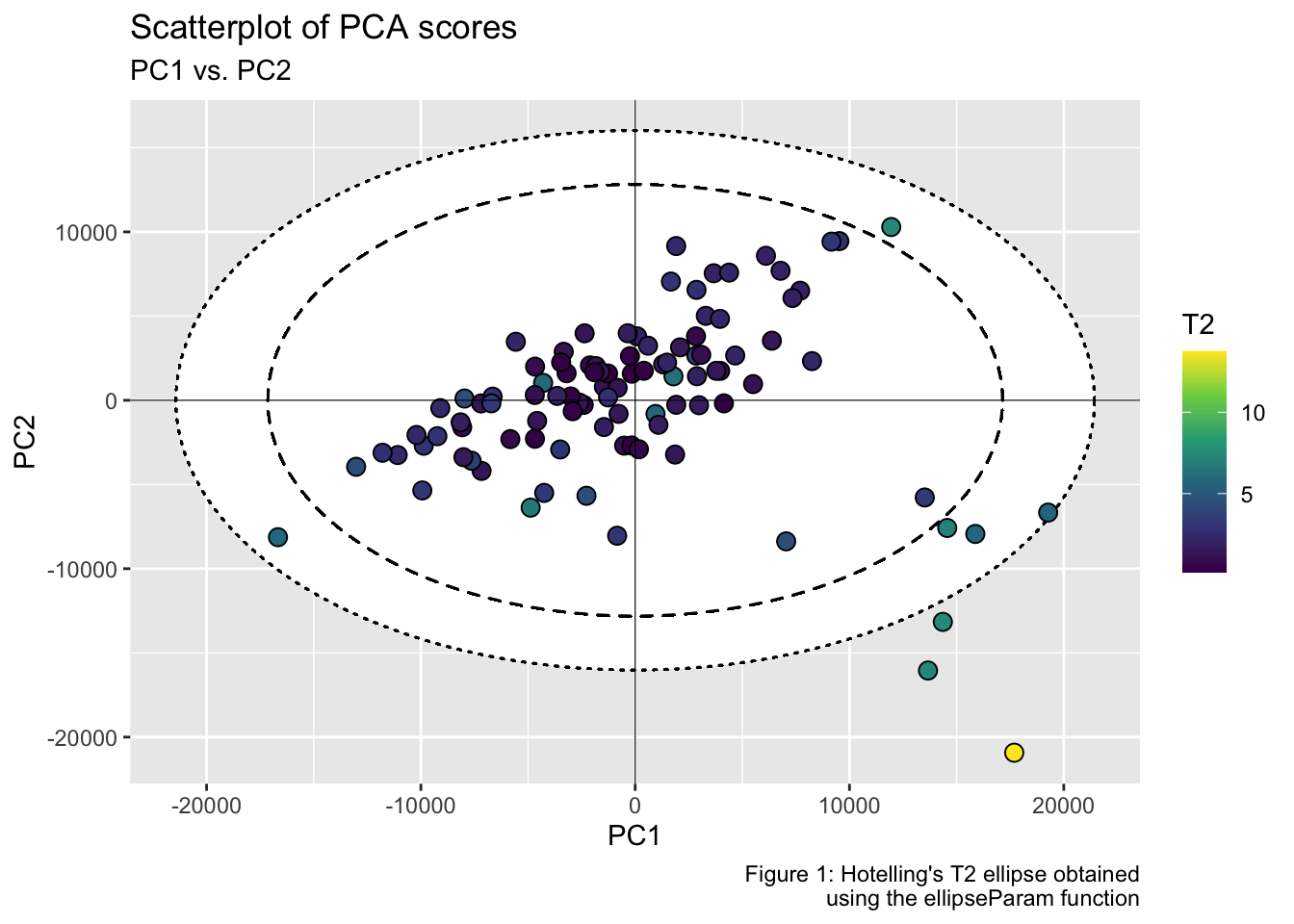
#> $ y: num [1:500] 8.73e-13 1.30e+02 2.59e+02 3.89e+02 5.19e+02 ...Step 6. Plot PC1 vs. PC2 scatterplot, with the two corresponding Hotelling ellipse. Points inside the two elliptical regions are within the 99% and 95% confidence intervals for the Hotelling’s T-squared.
pca_scores %>%
  ggplot(aes(x = Dim.1, y = Dim.2)) +
  geom_ellipse(aes(x0 = 0, y0 = 0, a = a1, b = b1, angle = 0), size = .5, linetype = "dotted", fill = "white") +
  geom_ellipse(aes(x0 = 0, y0 = 0, a = a2, b = b2, angle = 0), size = .5, linetype = "dashed", fill = "white") +
  geom_point(aes(fill = T2), shape = 21, size = 3, color = "black") +
  scale_fill_viridis_c(option = "viridis") +
  geom_hline(yintercept = 0, linetype = "solid", color = "black", size = .2) +
  geom_vline(xintercept = 0, linetype = "solid", color = "black", size = .2) +
  labs(title = "Scatterplot of PCA scores", subtitle = "PC1 vs. PC2", x = "PC1", y = "PC2", fill = "T2", caption = "Figure 1: Hotelling's T2 ellipse obtained\n using the ellipseParam function") +
  theme_grey()
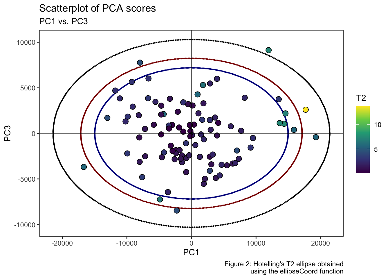
Or in the PC1-PC3 subspace at the confidence intervals set at 99, 95 and 90%.
ggplot() +
  geom_ellipse(data = coord_2PCs_99, aes(x0 = x, y0 = y, a = 1, b = 1, angle = 0), size = .9, color = "black", linetype = "dashed") +
  geom_ellipse(data = coord_2PCs_95, aes(x0 = x, y0 = y, a = 1, b = 1, angle = 0), size = .9, color = "darkred", linetype = "dotted") +
  geom_ellipse(data = coord_2PCs_90, aes(x0 = x, y0 = y, a = 1, b = 1, angle = 0), size = .9, color = "darkblue", linetype = "dotted") +
  geom_point(data = pca_scores, aes(x = Dim.1, y = Dim.3, fill = T2), shape = 21, size = 3, color = "black") +
  scale_fill_viridis_c(option = "viridis") +
  geom_hline(yintercept = 0, linetype = "solid", color = "black", size = .2) +
  geom_vline(xintercept = 0, linetype = "solid", color = "black", size = .2) +
  labs(title = "Scatterplot of PCA scores", subtitle = "PC1 vs. PC3", x = "PC1", y = "PC3", fill = "T2", caption = "Figure 2: Hotelling's T2 ellipse obtained\n using the ellipseCoord function") +
  theme_bw() +
  theme(panel.grid = element_blank())
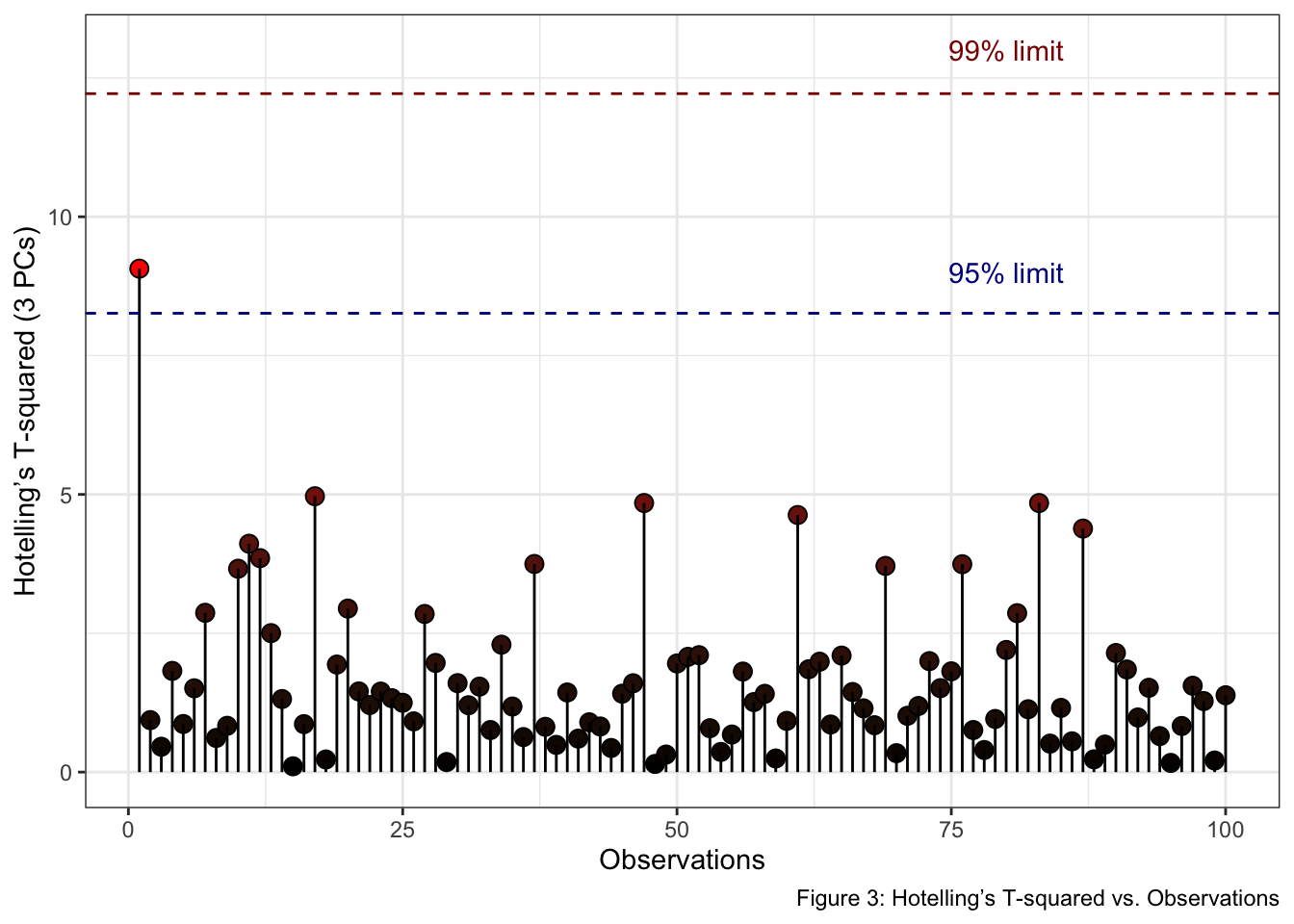
Note: The easiest way to analyze and interpret
Hotelling’s T-squared for more than two principal components, is to plot
Hotelling’s T-squared vs. Observations, where the confidence
limits are plotted as a line. Thus, observations below the two lines are
within the Hotelling’s T-squared limits. For example,
ellipseParam() is used with the first three principal
components (k = 3).
res_3PCs <- ellipseParam(data = pca_scores, k = 3)str(res_3PCs)
#> List of 3
#> $ Tsquare : tibble [100 × 1] (S3: tbl_df/tbl/data.frame)
#> ..$ value: num [1:100] 9.066 0.936 0.456 1.822 0.866 ...
#> $ cutoff.99pct: num 12.2
#> $ cutoff.95pct: num 8.26tibble(
T2 = pluck(res_3PCs, "Tsquare", "value"),
obs = 1:nrow(pca_scores)
) %>%
ggplot() +
geom_point(aes(x = obs, y = T2, fill = T2), shape = 21, size = 3, color = "black") +
geom_segment(aes(x = obs, y = T2, xend = obs, yend = 0), size = .5) +
scale_fill_gradient(low = "black", high = "red", guide = "none") +
geom_hline(yintercept = pluck(res_3PCs, "cutoff.99pct"), linetype = "dashed", color = "darkred", size = .5) +
geom_hline(yintercept = pluck(res_3PCs, "cutoff.95pct"), linetype = "dashed", color = "darkblue", size = .5) +
annotate("text", x = 80, y = 13, label = "99% limit", color = "darkred") +
annotate("text", x = 80, y = 9, label = "95% limit", color = "darkblue") +
labs(x = "Observations", y = "Hotelling’s T-squared (3 PCs)", fill = "T2 stats", caption = "Figure 3: Hotelling’s T-squared vs. Observations") +
theme_bw()