This package is designed to help the user specify, run, and then visualize and analyze the results of Ixodidae (hard-bodied ticks) population dynamics models. Such models exist in the literature, but the source code to run them is not always available. We wanted to provide an easy way for these models to be written and shared.
Install the package from CRAN with:
Here we provide a series of examples to help others see how models are specified and better understand the structure of the package. The examples highlight:
These examples all use and modify preset model configurations. If you wish to create a custom model configuration, see ?config().
We start with config_ex_1, a simple model configuration that doesn’t consider infection, and that has four life stages: __e for egg, __l for larvae, __n for nymph, and __a for adult.
We give a new range of parameter values for number of eggs laid.
eggs_laid <- c(800, 1000, 1200)
modified_configs <- vary_param(config_ex_1, from = '__a', to = '__e',
                               param_name = 'a', values = eggs_laid)
This gives us a list of three modified model configs, which differ only in the number of eggs laid.
outputs <- run_all_configs(modified_configs)
outputs[[1]]
#> # A tibble: 116 × 6
#>      day stage    pop age_group process infected
#>    <int> <chr>  <dbl> <chr>     <chr>   <lgl>
#>  1     1 __e        0 e         _       FALSE
#>  2     1 __l        0 l         _       FALSE
#>  3     1 __n        0 n         _       FALSE
#>  4     1 __a     1000 a         _       FALSE
#>  5     2 __e   800000 e         _       FALSE
#>  6     2 __l        0 l         _       FALSE
#>  7     2 __n        0 n         _       FALSE
#>  8     2 __a        0 a         _       FALSE
#>  9     3 __e        0 e         _       FALSE
#> 10     3 __l   800000 l         _       FALSE
#> # … with 106 more rows
The model output is a data frame where the column day indicates Julian date, stage indicates tick life stage, and pop is population size. The remaining columns breakdown the stage column into it’s constituent parts: the age and current process of a tick, and whether it is infected. Since we ran the model with multiple configurations, we get a list of data frames. Here we inspect only the first.
growth_rate() calculates the multiplicative growth rate for a model output. The population is stable with 1000 eggs laid, as indicated by the growth rate 1. The population decreases with 800 eggs laid, and increases with 1200 eggs laid.
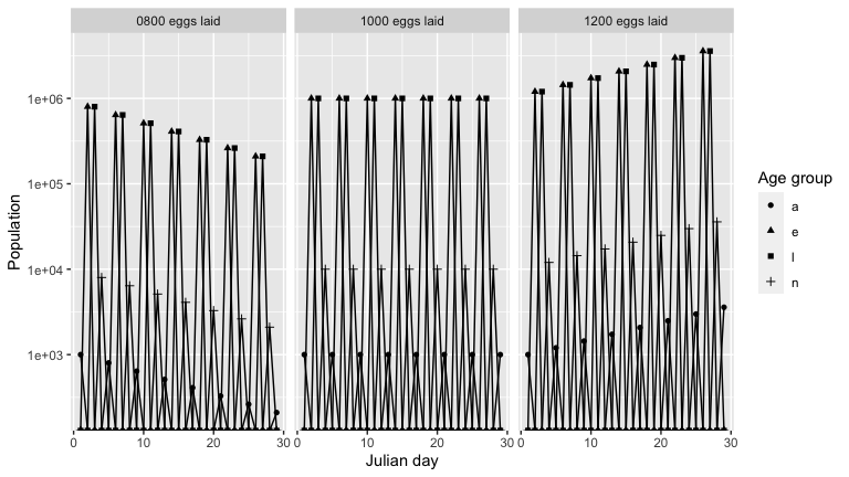
To see a breakdown of how the population is changing, we graph the population over time of each age group, for each model output. As expected, for each output there is a cycle with a peak in number of eggs, followed by peaks in larvae, nymph and then adult population.
names(outputs) <- c('0800 eggs laid', '1000 eggs laid', '1200 eggs laid')
outputs_stacked <- bind_rows(outputs, .id = "id")
outputs_stacked %>%
  graph_population_each_group() +
  facet_wrap(~ id)
temp_example_config$transitions
#> # A tibble: 16 × 7
#>    from  to    transition_fun delay source            pred1 pred2
#>    <chr> <chr> <chr>          <lgl> <chr>             <chr> <lgl>
#>  1 __e   q_l   expo_fun       TRUE  Ogden et al. 2004 temp  NA
#>  2 __e   m     constant_fun   TRUE  Ogden et al. 2005 <NA>  NA
#>  3 q_l   m     constant_fun   FALSE Ogden et al. 2005 <NA>  NA
#>  4 q_n   m     constant_fun   FALSE Ogden et al. 2005 <NA>  NA
#>  5 q_a   m     constant_fun   FALSE Ogden et al. 2005 <NA>  NA
#>  6 e_l   m     constant_fun   TRUE  Ogden et al. 2005 <NA>  NA
#>  7 e_n   m     constant_fun   TRUE  Ogden et al. 2005 <NA>  NA
#>  8 e_a   m     constant_fun   TRUE  Ogden et al. 2005 <NA>  NA
#>  9 r_a   m     constant_fun   FALSE Ogden et al. 2005 <NA>  NA
#> 10 q_l   e_l   constant_fun   FALSE <NA>              <NA>  NA
#> 11 e_l   q_n   expo_fun       TRUE  <NA>              temp  NA
#> 12 q_n   e_n   constant_fun   FALSE <NA>              <NA>  NA
#> 13 e_n   q_a   expo_fun       TRUE  <NA>              temp  NA
#> 14 q_a   e_a   constant_fun   FALSE <NA>              <NA>  NA
#> 15 e_a   r_a   expo_fun       TRUE  <NA>              temp  NA
#> 16 r_a   __e   constant_fun   FALSE <NA>              <NA>  NA
From the first line of this tick life-stage transitions table, you see that the development from eggs, __e, to questing larvae, q_l, is an exponential function of temperature. We can see the parameters for this transition:
temp_example_config$parameters %>% filter(from == '__e', to == 'q_l')
#> # A tibble: 2 × 8
#>   from  to    param_name host_spp param_value param_ci_low param_ci_high source
#>   <chr> <chr> <chr>      <lgl>          <dbl> <lgl>        <lgl>         <chr>
#> 1 __e   q_l   a          NA         0.0000292 NA           NA            Ogden …
#> 2 __e   q_l   b          NA         2.27      NA           NA            Ogden …
The daily development rate is 0.0000292*temp^2.27.
Here we highlight how this temperature dependence affects the output of the model. We make a second config in which the daily temperature is one degree warmer.
cfg2 <- temp_example_config
cfg2$weather <- temp_example_config$predictors %>% mutate(value = value + 1)

output1 <- run(temp_example_config)
output2 <- run(cfg2)

output1 <- output1 %>% mutate(temp = 'cold')
output2 <- output2 %>% mutate(temp = 'warm')
Finally, we compare the outputs for a commonly measured aspect of tick populations, the number of questing nymphs.
output1 %>%
  rbind(output2) %>%
  filter(stage == 'q_n') %>%
  ggplot(aes(day, pop, col = temp)) +
  geom_line() +
  scale_color_manual(values = c('cold' = 'blue', 'warm' = 'red')) +
  ylab('Questing nymphs')
Here you can see nymphs start questing earlier and reach a higher population in the warmer climate.
In the previous example there was no host community explicitly stated and ticks had a constant probability of transition between life stages (e.g., from larva to nymph). It is possible to instead model these probabilities based on host community composition.
host_example_config$transitions
#> # A tibble: 16 × 7
#>    from  to    transition_fun delay source            pred1    pred2
#>    <chr> <chr> <chr>          <lgl> <chr>             <chr>    <lgl>
#>  1 __e   q_l   expo_fun       TRUE  Ogden et al. 2004 temp     NA
#>  2 __e   m     constant_fun   TRUE  Ogden et al. 2005 <NA>     NA
#>  3 q_l   m     constant_fun   FALSE Ogden et al. 2005 <NA>     NA
#>  4 q_n   m     constant_fun   FALSE Ogden et al. 2005 <NA>     NA
#>  5 q_a   m     constant_fun   FALSE Ogden et al. 2005 <NA>     NA
#>  6 e_l   m     constant_fun   TRUE  Ogden et al. 2005 <NA>     NA
#>  7 e_n   m     constant_fun   TRUE  Ogden et al. 2005 <NA>     NA
#>  8 e_a   m     constant_fun   TRUE  Ogden et al. 2005 <NA>     NA
#>  9 r_a   m     constant_fun   FALSE Ogden et al. 2005 <NA>     NA
#> 10 q_l   e_l   find_n_feed    FALSE <NA>              host_den NA
#> 11 e_l   q_n   expo_fun       TRUE  <NA>              temp     NA
#> 12 q_n   e_n   find_n_feed    FALSE <NA>              host_den NA
#> 13 e_n   q_a   expo_fun       TRUE  <NA>              temp     NA
#> 14 q_a   e_a   find_n_feed    FALSE <NA>              host_den NA
#> 15 e_a   r_a   expo_fun       TRUE  <NA>              temp     NA
#> 16 r_a   __e   constant_fun   FALSE <NA>              <NA>     NA
Here transition from questing larvae, q_l, to engorged larvae, e_l, depends on the host_den, which is how the host community is included in the transition.
host_example_config$parameters %>% filter(from == 'q.l', to == 'e.l')
#> # A tibble: 6 × 8
#>   from  to    param_name  host_spp param_value param_ci_low param_ci_high source
#>   <chr> <chr> <chr>       <chr>          <dbl> <lgl>        <lgl>         <chr>
#> 1 q.l   e.l   pref        deer            0.25 NA           NA            <NA>
#> 2 q.l   e.l   feed_succe… deer            0.49 NA           NA            Levi …
#> 3 q.l   e.l   pref        mouse           1    NA           NA            <NA>
#> 4 q.l   e.l   feed_succe… mouse           0.49 NA           NA            Levi …
#> 5 q.l   e.l   pref        squirrel        0.25 NA           NA            <NA>
#> 6 q.l   e.l   feed_succe… squirrel        0.17 NA           NA            Levi …
Here the parameters of find_n_feed get different values for each host species. In this case the two parameters are pref, which is the larval tick’s preference for the three different host species, and feed_success, which is the fraction of feeding larvae which successfully feed to completion.
In this example the temperature and host community are constant through time, but the package also supports variable temperature and host community data to see how seasonal or year-to-year variation in affects tick populations.
We now compare how different host densities affect tick populations. Here we vary the deer density.
cfg_lowdeerden <- host_example_config
cfg_highdeerden <- host_example_config
cfg_lowdeerden$predictors <- host_example_config$predictors %>%
  mutate(value = ifelse(pred == 'host_den' & pred_subcategory == 'deer', 0.1, value))
cfg_highdeerden$predictors <- host_example_config$predictors %>%
  mutate(value = ifelse(pred == 'host_den' & pred_subcategory == 'deer', 5, value))


output_middeerden <- run(host_example_config)
output_lowdeerden <- run(cfg_lowdeerden)
output_highdeerden <- run(cfg_highdeerden)

output_middeerden <- output_middeerden %>% mutate(deer_den = 'mid')
output_lowdeerden <- output_lowdeerden %>% mutate(deer_den = 'low')
output_highdeerden <- output_highdeerden %>% mutate(deer_den = 'high')
And then use the graph_population_each_group() function to see how the deer densities affect the tick population.
output_lowdeerden %>%
  bind_rows(output_middeerden, output_highdeerden) %>%
  mutate(deer_den = factor(deer_den, levels = c('low', 'mid', 'high'))) %>%
  graph_population_each_group() +
  facet_wrap(~deer_den)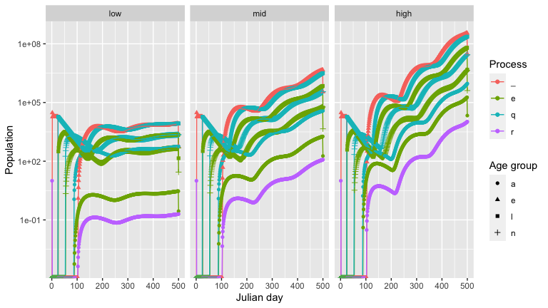
In the examples above we modeled a tick population without a tick borne disease. Here we give an example of how the package can be used to also include infection dynamics.
So far all examples have used transition functions loaded into the package, here we show how to define our own.
infect_example_config$transitions
#> # A tibble: 33 × 6
#>    from  to    transition_fun delay pred1    pred2
#>    <chr> <chr> <chr>          <lgl> <chr>    <lgl>
#>  1 __e   q_l   constant_fun   TRUE  <NA>     NA
#>  2 __e   m     constant_fun   TRUE  <NA>     NA
#>  3 q_l   f_l   find_host      FALSE host_den NA
#>  4 q_l   m     constant_fun   FALSE <NA>     NA
#>  5 f_l   eil   infect_fun     FALSE host_den NA
#>  6 f_l   eul   infect_fun     FALSE host_den NA
#>  7 eil   qin   constant_fun   TRUE  <NA>     NA
#>  8 eil   m     constant_fun   TRUE  <NA>     NA
#>  9 eul   qun   constant_fun   TRUE  <NA>     NA
#> 10 eul   m     constant_fun   TRUE  <NA>     NA
#> # … with 23 more rows
Here we use the middle character of the life-stage key. It is either i for infected or u for uninfected. We assume no transovarial infection so questing larvae are uninfected. But after they feed, f_l, they can either become engorged infected, eil, or engorged uninfected, eul, larvae. This is based on infect_fun, which as above has host species-specific parameters of pref and host_rc (reservoir competence).
Deer are important to the blacklegged tick as the main host of adult ticks. As such they are thought to increase tick populations (see above). But deer can also serve as hosts for juvenile tick life stages, and deer are poor reservoirs for Borrelia burgdorferi. So increased deer density may also decrease the proportion of bloodmeals juvenile ticks take from more competent reservoirs life mice. We use this simple model to illustrate this possibility.
deer_den <- c(0.1, 0.25, 0.5, 0.75, 1)
results_tib <- tibble(deer = deer_den, nymph_den = 0, nip = 0)

for (i in 1:5)
{
  cfg_mod <- infect_example_config
  cfg_mod$predictors[1,4] <- deer_den[i]
  out <- run(cfg_mod)

  nymph_sum <- out %>%
  filter(stage == 'qin' | stage == 'qun') %>%
  group_by(stage) %>%
  summarise(totpop = sum(pop))

  results_tib$nip[i] <- unlist(nymph_sum[1,2] /(nymph_sum[1,2] + nymph_sum[2,2]))
  results_tib$nymph_den[i] <- out %>%
    filter(stage == 'qin' | stage == 'qun') %>%
    summarise(totpop = sum(pop)) %>%
    unlist()
}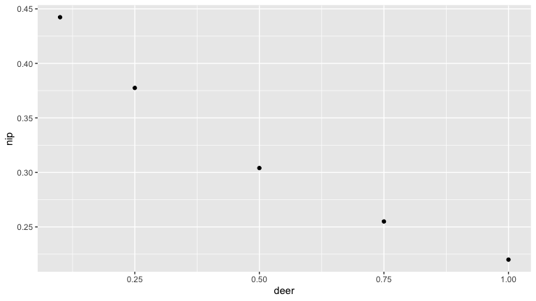

Here we see that as deer density increases the number of nymphs increases (as the tick population gets bigger). But the nymph infection prevalence (NIP) goes down.