author: Jacek Białek, University of Lodz, Statistics Poland
Goals of PriceIndices are as follows: a) data processing before price index calculations; b) bilateral and multilateral price index calculations; c) extending multilateral price indices. You can download the package documentation from here.
You can install the released version of PriceIndices from CRAN with:
install.packages("PriceIndices")You can install the development version of PriceIndices from GitHub with:
library("remotes")
remotes::install_github("JacekBialek/PriceIndices")This package includes seven data sets: artificial and real.
1) dataAGGR
The first one, dataAGGR, can be used to demonstrate the data_aggregating function. This is a collection of artificial scanner data on milk products sold in three different months and it contains the following columns: time - dates of transactions (Year-Month-Day: 4 different dates); prices - prices of sold products (PLN); quantities - quantities of sold products (liters); prodID - unique product codes (3 different prodIDs); retID - unique codes identifying outlets/retailer sale points (4 different retIDs); description - descriptions of sold products (two subgroups: goat milk, powdered milk).
2) dataMATCH
The second one, dataMATCH, can be used to demonstrate the data_matching function and it will be described in the next part of the guidelines. Generally, this artificial data set contains the following columns: time - dates of transactions (Year-Month-Day); prices - prices of sold products; quantities - quantities of sold products; codeIN - internal product codes from the retailer; codeOUT - external product codes, e.g. GTIN or SKU in the real case; description - descriptions of sold products, eg. ‘product A’, ‘product B’, etc.
3) dataCOICOP
The third one, dataCOICOP, is a ollection of real scanner data on the sale of milk products sold in a period: Dec, 2020 - Feb, 2022. It is a data frame with 10 columns and 139600 rows. The used variables are as follows: time - dates of transactions (Year-Month-Day); prices - prices of sold products (PLN); quantities - quantities of sold products; description - descriptions of sold products (original: in Polish); codeID - retailer product codes; grammage - product grammages, unit - sales units, e.g. ‘kg’, ‘ml’, etc.; category - product categories (in English) corresponding to COICOP 6 levels, coicop6 - identifiers of local COICOP 6 groups (6 levels). Please note that this data set can serve as a training or testing set in product classification using machine learning methods (see the functions: model_classification and data_classifying).
4) milk
This data set, milk, is a collection of scaner data on the sale of milk in one of Polish supermarkets in the period from December 2018 to August 2020. It is a data frame with 6 columns and 4386 rows. The used variables are as follows: time - dates of transactions (Year-Month-Day); prices - prices of sold products (PLN); quantities - quantities of sold products (liters); prodID - unique product codes obtained after product matching (data set contains 68 different prodIDs); retID - unique codes identifying outlets/retailer sale points (data set contains 5 different retIDs); description - descriptions of sold milk products (data set contains 6 different product descriptions corresponding to subgroups of the milk group).
5) coffee
This data set, coffee, is a collection of scanner data on the sale of coffee in one of Polish supermarkets in the period from December 2017 to October 2020. It is a data frame with 6 columns and 42561 rows. The used variables are as follows: time - dates of transactions (Year-Month-Day); prices - prices of sold products (PLN); quantities - quantities of sold products (kg); prodID - unique product codes obtained after product matching (data set contains 79 different prodIDs); retID - unique codes identifying outlets/retailer sale points (data set contains 20 different retIDs); description - descriptions of sold coffee products (data set contains 3 different product descriptions corresponding to subgroups of the coffee group).
6) sugar
This data set, sugar, is a collection of scanner data on the sale of coffee in one of Polish supermarkets in the period from December 2017 to October 2020. It is a data frame with 6 columns and 7666 rows. The used variables are as follows: time - dates of transactions (Year-Month-Day); prices - prices of sold products (PLN); quantities - quantities of sold products (kg); prodID - unique product codes obtained after product matching (data set contains 11 different prodIDs); retID - unique codes identifying outlets/retailer sale points (data set contains 20 different retIDs); description - descriptions of sold sugar products (data set contains 3 different product descriptions corresponding to subgroups of the sugar group).
7) dataU
This data set, dataU, is a collection of artificial scanner data on 6 products sold in Dec, 2018. Product descriptions contain the information about their grammage and unit. It is a data frame with 5 columns and 6 rows. The used variables are as follows: time - dates of transactions (Year-Month-Day); prices - prices of sold products (PLN); quantities - quantities of sold products (item); prodID - unique product codes; description - descriptions of sold products (data set contains 6 different product descriptions).
The set milk represents a typical data frame used in the package for most calculations and is organized as follows:
library(PriceIndices)
head(milk)
#>         time prices quantities prodID retID   description
#> 1 2018-12-01   8.78        9.0  14215  2210 powdered milk
#> 2 2019-01-01   8.78       13.5  14215  2210 powdered milk
#> 3 2019-02-01   8.78        0.5  14215  1311 powdered milk
#> 4 2019-02-01   8.78        8.0  14215  2210 powdered milk
#> 5 2019-03-01   8.78        0.5  14215  1311 powdered milk
#> 6 2019-03-01   8.78        1.5  14215  2210 powdered milk
Available subgroups of sold milk are
unique(milk$description)
#> [1] "powdered milk"             "low-fat milk pasteurized"
#> [3] "low-fat milk UHT"          "full-fat milk pasteurized"
#> [5] "full-fat milk UHT"         "goat milk"
Generating artificial scanner data sets in the package
The package includes the generate function which provides an artificial scanner data sets where prices and quantities are lognormally distributed. The characteristics for these lognormal distributions are set by pmi, sigma, qmi and qsigma parameters. This function works for the fixed number of products and outlets (see n and r parameters). The generated data set is ready for further price index calculations. For instance:
dataset<-generate(pmi=c(1.02,1.03,1.04),psigma=c(0.05,0.09,0.02),
                  qmi=c(3,4,4),qsigma=c(0.1,0.1,0.15),
                  start="2020-01")
head(dataset)
#>         time prices quantities prodID retID
#> 1 2020-01-01   2.78         17      1     1
#> 2 2020-01-01   2.64         19      2     1
#> 3 2020-01-01   2.70         20      3     1
#> 4 2020-01-01   2.82         21      4     1
#> 5 2020-01-01   2.69         17      5     1
#> 6 2020-01-01   2.82         21      6     1
From the other hand you can use tindex function to obtain the theoretical value of the unweighted price index for lognormally distributed prices (the month defined by start parameter plays a role of the fixed base period). The characteristics for these lognormal distributions are set by pmi and sigma parameters. The ratio parameter is a logical parameter indicating how we define the theoretical unweighted price index. If it is set to TRUE then the resulting value is a ratio of expected price values from compared months; otherwise the resulting value is the expected value of the ratio of prices from compared months.The function provides a data frame consisting of dates and corresponding expected values of the theoretical unweighted price index. For example:
tindex(pmi=c(1.02,1.03,1.04),psigma=c(0.05,0.09,0.02),start="2020-01",ratio=FALSE)
#>      date   tindex
#> 1 2020-01 1.000000
#> 2 2020-02 1.012882
#> 3 2020-03 1.019131data_preparing
This function returns a prepared data frame based on the user’s data set (you can check if your data set it is suitable for further price index calculation by using data_check function). The resulting data frame is ready for further data processing (such as data selecting, matching or filtering) and it is also ready for price index calculations (if only it contains the required columns). The resulting data frame is free from missing values, zero or negative prices and quantities. As a result, the column time is set to be Date type (in format: ‘Year-Month-01’), while the columns prices and quantities are set to be numeric. If the description parameter is set to TRUE then the column description is set to be character type (otherwise it is deleted). Please note that the milk set is an already prepared dataset but let us assume for a moment that we want to make sure that it does not contain missing values and we do not need the column description for further calculations. For this purpose, we use the data_preparing function as follows:
head(data_preparing(milk, time="time",prices="prices",quantities="quantities"))
#>         time prices quantities
#> 1 2018-12-01   8.78        9.0
#> 2 2019-01-01   8.78       13.5
#> 3 2019-02-01   8.78        0.5
#> 4 2019-02-01   8.78        8.0
#> 5 2019-03-01   8.78        0.5
#> 6 2019-03-01   8.78        1.5
data_aggregating
The function aggregates the user’s data frame over time and/or over outlets. Consequently, we obtain monthly data, where the unit value is calculated instead of a price for each prodID observed in each month (the time column gets the Date format: “Year-Month-01”). If paramter join_outlets is TRUE, then the function also performs aggregation over outlets (retIDs) and the retID column is removed from the data frame. The main advantage of using this function is the ability to reduce the size of the data frame and the time needed to calculate the price index. For instance, let us consider the following data set:
dataAGGR
#>         time prices quantities prodID retID   description
#> 1 2018-12-01     10        100 400032  4313     goat milk
#> 2 2018-12-01     15        100 400032  1311     goat milk
#> 3 2018-12-01     20        100 400032  1311     goat milk
#> 4 2020-07-01     20        100 400050  1311     goat milk
#> 5 2020-08-01     30         50 400050  1311     goat milk
#> 6 2020-08-01     40         50 400050  2210     goat milk
#> 7 2018-12-01     15        200 403249  2210 powdered milk
#> 8 2018-12-01     15        200 403249  2210 powdered milk
#> 9 2018-12-01     15        300 403249  2210 powdered milk
After aggregating this data set over time and outlets we obtain:
data_aggregating(dataAGGR)
#>         time prices quantities prodID   description
#> 1 2018-12-01     15        300 400032     goat milk
#> 2 2018-12-01     15        700 403249 powdered milk
#> 3 2020-07-01     20        100 400050     goat milk
#> 4 2020-08-01     35        100 400050     goat milk
data_unit
The function returns the user’s data frame with two additional columns: grammage and unit (both are character type). The values of these columns are extracted from product descriptions on the basis of provided units. Please note, that the function takes into consideration a sign of the multiplication, e.g. if the product description contains: ‘2x50 g’, we will obtain: grammage: 100 and unit: g for that product (for multiplication set to ‘x’). For example:
data_unit(dataU,units=c("g","ml","kg","l"),multiplication="x")
#>         time prices quantities prodID          description grammage unit
#> 1 2018-12-01   8.00        200  40033 drink 0,75l 3% corma     0.75    l
#> 2 2018-12-01   5.20        300  12333          sugar 0.5kg      0.5   kg
#> 3 2018-12-01  10.34        100  20345         milk 4x500ml     2000   ml
#> 4 2018-12-01   2.60        500  15700 xyz 3 4.34 xyz 200 g      200    g
#> 5 2018-12-01  12.00       1000  13022                  abc        1 item
#> 6 2019-01-01   3.87        250  10011     ABC 2A/350 g mnk      350    g
data_norm
The function returns the user’s data frame with two transformed columns: grammage and unit, and two rescaled columns: prices and quantities. The above-mentioned transformation and rescaling take into consideration the user rules. Recalculated prices and quantities concern grammage units defined as the second parameter in the given rule. For instance:
# Preparing a data set
data<-data_unit(dataU,units=c("g","ml","kg","l"),multiplication="x")
# Normalization of grammage units
data_norm(data, rules=list(c("ml","l",1000),c("g","kg",1000)))
#>         time   prices quantities prodID          description grammage unit
#> 1 2018-12-01  5.17000      200.0  20345         milk 4x500ml        2    l
#> 2 2018-12-01 10.66667      150.0  40033 drink 0,75l 3% corma     0.75    l
#> 3 2018-12-01 13.00000      100.0  15700 xyz 3 4.34 xyz 200 g      0.2   kg
#> 4 2019-01-01 11.05714       87.5  10011     ABC 2A/350 g mnk     0.35   kg
#> 5 2018-12-01 10.40000      150.0  12333          sugar 0.5kg      0.5   kg
#> 6 2018-12-01 12.00000     1000.0  13022                  abc        1 item
data_selecting
The function returns a subset of the user’s data set obtained by selection based on keywords and phrases defined by parameters: include, must and exclude (an additional column coicop is optional). Providing values of these parameters, please remember that the procedure distinguishes between uppercase and lowercase letters only when sensitivity is set to TRUE.
For instance, please use
subgroup1<-data_selecting(milk, include=c("milk"), must=c("UHT"))
head(subgroup1)
#>         time prices quantities prodID retID      description
#> 1 2018-12-01   2.97         78  17034  1311 low-fat milk uht
#> 2 2018-12-01   2.97        167  17034  2210 low-fat milk uht
#> 3 2018-12-01   2.97        119  17034  6610 low-fat milk uht
#> 4 2018-12-01   2.97         32  17034  7611 low-fat milk uht
#> 5 2018-12-01   2.97         54  17034  8910 low-fat milk uht
#> 6 2019-01-01   2.95         71  17034  1311 low-fat milk uht
to obtain the subset of milk limited to UHT category:
unique(subgroup1$description)
#> [1] "low-fat milk uht"  "full-fat milk uht"
You can use
subgroup2<-data_selecting(milk, must=c("milk"), exclude=c("past","goat"))
head(subgroup2)
#>         time prices quantities prodID retID   description
#> 1 2018-12-01   8.78        9.0  14215  2210 powdered milk
#> 2 2019-01-01   8.78       13.5  14215  2210 powdered milk
#> 3 2019-02-01   8.78        0.5  14215  1311 powdered milk
#> 4 2019-02-01   8.78        8.0  14215  2210 powdered milk
#> 5 2019-03-01   8.78        0.5  14215  1311 powdered milk
#> 6 2019-03-01   8.78        1.5  14215  2210 powdered milk
to obtain the subset of milk with products which are not pasteurized and which are not goat:
unique(subgroup2$description)
#> [1] "powdered milk"     "low-fat milk uht"  "full-fat milk uht"
data_classifying
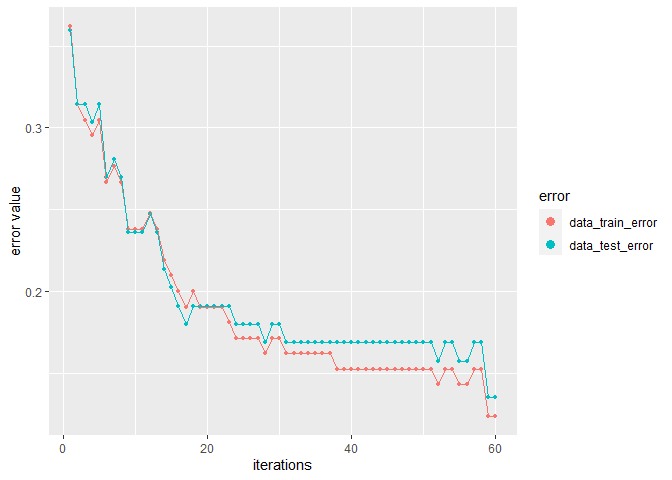
This function predicts product COICOP levels (or any other defined product levels) using the selected machine learning model (see the model parameter). It provides the indicated data set with an additional column, i.e. coicop_predicted. The selected model must be built previously (see the model_classification function) and after the training process it can be saved on your disk (see the save_model function) and then loaded at any time (see the load_model function). Please note that the machine learning process is based on the XGBoost algorithm (from the XGBoost package) which is an implementation of gradient boosted decision trees designed for speed and performance. For example, let us build a machine learning model
my.grid=list(eta=c(0.01,0.02,0.05),subsample=c(0.5,0.8))
data_train<-dplyr::filter(dataCOICOP,dataCOICOP$time<=as.Date("2021-10-01"))
data_test<-dplyr::filter(dataCOICOP,dataCOICOP$time==as.Date("2021-11-01"))
ML<-model_classification(data_train,
                         data_test,
                         coicop="coicop6",
                         grid=my.grid,
                         indicators=c("description","codeIN"),
                         key_words=c("uht"),
                         rounds=60)
We can watch the results of the whole training process:
ML$figure_training
or we can observe the importance of the used indicators:
ML$figure_importance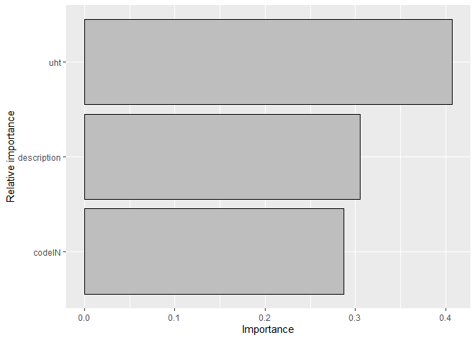
Now, let us save the model on the disk. After saving the model we can load it and use at any time:
#Setting a temporary directory as a working directory
wd<-tempdir()
setwd(wd)
#Saving and loading the model
save_model(ML, dir="My_model")
ML_fromPC<-load_model("My_model")
#Prediction
data_predicted<-data_classifying(ML_fromPC, data_test)
head(data_predicted)
#>         time prices quantities                            description codeIN
#> 1 2021-11-01   3.03        379 g/wydojone mleko bez laktozyuht 3,2%1l  60001
#> 2 2021-11-01   3.03        856 g/wydojone mleko bez laktozyuht 3,2%1l  60001
#> 3 2021-11-01   3.03        369 g/wydojone mleko bez laktozyuht 3,2%1l  60001
#> 4 2021-11-01   3.03        617 g/wydojone mleko bez laktozyuht 3,2%1l  60001
#> 5 2021-11-01   3.03        613 g/wydojone mleko bez laktozyuht 3,2%1l  60001
#> 6 2021-11-01   3.03        261 g/wydojone mleko bez laktozyuht 3,2%1l  60001
#>   retID grammage unit       category coicop6 coicop_predicted
#> 1     2        1    l UHT whole milk 11411_1          11411_1
#> 2     3        1    l UHT whole milk 11411_1          11411_1
#> 3     4        1    l UHT whole milk 11411_1          11411_1
#> 4     5        1    l UHT whole milk 11411_1          11411_1
#> 5     6        1    l UHT whole milk 11411_1          11411_1
#> 6     7        1    l UHT whole milk 11411_1          11411_1
data_matching
If you have a dataset with information about products sold but they are not matched you can use the data_matching function. In an optimal situation, your data frame contains the codeIN, codeOUT and description columns (see documentation), which in practice will contain retailer codes, GTIN or SKU codes and product labels, respectively. The data_matching function returns a data set defined in the first parameter (data) with an additional column (prodID). Two products are treated as being matched if they have the same prodID value. The procedure of generating the above-mentioned additional column depends on the set of chosen columns for matching (see documentation for details). For instance, let us suppose you want to obtain matched products from the following, artificial data set:
head(dataMATCH)
#>         time    prices quantities codeIN codeOUT retID description
#> 1 2018-12-01  9.416371        309      1       1     1   product A
#> 2 2019-01-01  9.881875        325      1       5     1   product A
#> 3 2019-02-01 12.611826        327      1       1     1   product A
#> 4 2018-12-01  9.598252        309      3       2     1   product A
#> 5 2019-01-01  9.684900        325      3       2     1   product A
#> 6 2019-02-01  9.358420        327      3       2     1   product A
Let us assume that products with two identical codes (codeIN and codeOUT) or one of the codes identical and an identical description are automatically matched. Products are also matched if they have one of the codes identical and the Jaro-Winkler distance of their descriptions is bigger than the fixed precision value (see documentation - Case 1). Let us also suppose that you want to match all products sold in the interval: December 2018 - February 2019. If you use the data_matching function (as below), an additional column (prodID) will be added to your data frame:
data1<-data_matching(dataMATCH, start="2018-12",end="2019-02", codeIN=TRUE, codeOUT=TRUE, precision=.98, interval=TRUE)
head(data1)
#>         time    prices quantities codeIN codeOUT retID description prodID
#> 1 2018-12-01  9.416371        309      1       1     1   product A      4
#> 2 2019-01-01  9.881875        325      1       5     1   product A      4
#> 3 2019-02-01 12.611826        327      1       1     1   product A      4
#> 4 2018-12-01  9.598252        309      3       2     1   product A      9
#> 5 2019-01-01  9.684900        325      3       2     1   product A      9
#> 6 2019-02-01  9.358420        327      3       2     1   product A      9
Let us now suppose you do not want to consider codeIN while matching and that products with an identical description are to be matched too:
data2<-data_matching(dataMATCH, start="2018-12",end="2019-02",
                     codeIN=FALSE, onlydescription=TRUE, interval=TRUE)
head(data2)
#>         time    prices quantities codeIN codeOUT retID description prodID
#> 1 2018-12-01  9.416371        309      1       1     1   product A      7
#> 2 2019-01-01  9.881875        325      1       5     1   product A      7
#> 3 2019-02-01 12.611826        327      1       1     1   product A      7
#> 4 2018-12-01  9.598252        309      3       2     1   product A      7
#> 5 2019-01-01  9.684900        325      3       2     1   product A      7
#> 6 2019-02-01  9.358420        327      3       2     1   product A      7
Now, having a prodID column, your datasets are ready for further price index calculations, e.g.:
fisher(data1, start="2018-12", end="2019-02")
#> [1] 1.018419
jevons(data2, start="2018-12", end="2019-02")
#> [1] 1.074934
data_filtering
This function returns a filtered data set, i.e. a reduced user’s data frame with the same columns and rows limited by a criterion defined by the filters parameter (see documentation). If the set of filters is empty then the function returns the original data frame (defined by the data parameter). On the other hand, if all filters are chosen, i.e. filters=c(extremeprices, dumpprices, lowsales), then these filters work independently and a summary result is returned. Please note that both variants of the extremeprices filter can be chosen at the same time, i.e. plimits and pquantiles, and they work also independently. For example, let us assume we consider three filters: filter1 is to reject 1% of the lowest and 1% of the highest price changes comparing March 2019 to December 2018, filter2 is to reject products with the price ratio being less than 0.5 or bigger than 2 in the same time, filter3 rejects the same products as filter2 rejects and also products with relatively low sale in compared months, filter4 rejects products with the price ratio being less than 0.9 and with the expenditure ratio being less than 0.8 in the same time.
filter1<-data_filtering(milk,start="2018-12",end="2019-03",
                        filters=c("extremeprices"),pquantiles=c(0.01,0.99))
filter2<-data_filtering(milk,start="2018-12",end="2019-03",
                        filters=c("extremeprices"),plimits=c(0.5,2))
filter3<-data_filtering(milk,start="2018-12",end="2019-03",
                        filters=c("extremeprices","lowsales"),plimits=c(0.5,2))
filter4<-data_filtering(milk,start="2018-12",end="2019-03",
                        filters=c("dumpprices"),dplimits=c(0.9,0.8))
These three filters differ from each other with regard to the data reduction level:
data_without_filters<-data_filtering(milk,start="2018-12",end="2019-03",filters=c())
nrow(data_without_filters)
#> [1] 413
nrow(filter1)
#> [1] 378
nrow(filter2)
#> [1] 381
nrow(filter3)
#> [1] 170
nrow(filter4)
#> [1] 374
You can also use data_filtering for each pair of subsequent months from the considered time interval under the condition that this filtering is done for each outlet (retID) separately, e.g.
filter1B<-data_filtering(milk,start="2018-12",end="2019-03",
                         filters=c("extremeprices"),pquantiles=c(0.01,0.99),
                         interval=TRUE, retailers=TRUE)
nrow(filter1B)
#> [1] 773available
The function returns all values from the indicated column (defined by the type parameter) which occur at least once in one of compared periods or in a given time interval. Possible values of the type parameter are: retID, prodID, codeIN, codeOUT or description (see documentation). If the interval parameter is set to FALSE, then the function compares only periods defined by period1 and period2. Otherwise the whole time period between period1 and period2 is considered. For example:
available(milk, period1="2018-12", period2="2019-12", type="retID",interval=TRUE)
#> [1] 2210 1311 6610 7611 8910
matched
The function returns all values from the indicated column (defined by the type parameter) which occur simultaneously in the compared periods or in a given time interval.Possible values of the type parameter are: retID, prodID, codeIN, codeOUT or description (see documentation). If the interval parameter is set to FALSE, then the function compares only periods defined by period1 and period2. Otherwise the whole time period between period1 and period2 is considered. For example:
matched(milk, period1="2018-12", period2="2019-12", type="prodID",interval=TRUE)
#>  [1]  14216  15404  17034  34540  60010  70397  74431  82827  82830  82919
#> [11]  94256 400032 400033 400189 400194 400195 400196 401347 401350 402263
#> [21] 402264 402293 402569 402570 402601 402602 402609 403249 404004 404005
#> [31] 405419 405420 406223 406224 406245 406246 406247 407219 407220 407669
#> [41] 407670 407709 407859 407860 400099
matched_index
The function returns a ratio of values from the indicated column that occur simultaneously in the compared periods or in a given time interval to all available values from the above-mentioned column (defined by the type parameter) at the same time. Possible values of the type parameter are: retID, prodID, codeIN, codeOUT or description (see documentation). If the interval parameter is set to FALSE, then the function compares only periods defined by period1 and period2. Otherwise the whole time period between period1 and period2 is considered. The returned value is from 0 to 1. For example:
matched_index(milk, period1="2018-12", period2="2019-12", type="prodID",interval=TRUE)
#> [1] 0.7258065
matched_fig
The function returns a data frame or a figure presenting the matched_index function calculated for the column defined by the type parameter and for each month from the considered time interval. The interval is set by the start and end parameters. The returned object (data frame or figure) depends on the value of the figure parameter. Examples:
matched_fig(milk, start="2018-12", end="2019-12", type="prodID")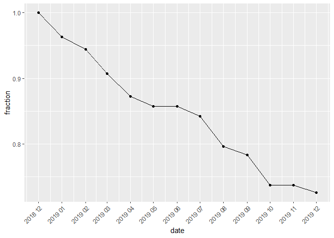
matched_fig(milk, start="2018-12", end="2019-04", type="prodID", figure=FALSE)
#>      date  fraction
#> 1 2018-12 1.0000000
#> 2 2019-01 0.9629630
#> 3 2019-02 0.9444444
#> 4 2019-03 0.9074074
#> 5 2019-04 0.8727273
prices
The function returns prices (unit value) of products with a given ID (prodID column) and being sold in the time period indicated by the period parameter. The set parameter means a set of unique product IDs to be used for determining prices of sold products. If the set is empty the function returns prices of all products being available in the period. To get prices (unit values) of all available milk products sold in July, 2019, please use:
prices(milk, period="2019-06")
#>  [1]  8.700000  8.669455  1.890000  2.950000  1.990000  2.990000  2.834464
#>  [8]  4.702051  2.163273  2.236250  2.810000  2.860000  2.400000  2.588644
#> [15]  3.790911  7.980000 64.057143 18.972121 12.622225  9.914052  7.102823
#> [22]  3.180000  2.527874  1.810000  1.650548  2.790000  2.490000  2.590000
#> [29]  7.970131  9.901111 15.266667 19.502286  2.231947  2.674401  2.371819
#> [36]  2.490000  6.029412  6.441176  2.090000  1.990000  1.890000  1.450000
#> [43]  2.680000  2.584184  2.683688  2.390000  3.266000  2.813238  7.966336
quantities
The function returns quantities of products with a given ID (prodID column) and being sold in the time period indicated by the period parameter. The set parameter means a set of unique product IDs to be used for determining prices of sold products. If the set is empty the function returns quantities of all products being available in the period. To get quantities of milk products with prodIDs: 400032, 71772 and 82919, and sold in July, 2019, please use:
quantities(milk, period="2019-06", set=c(400032, 71772, 82919))
#> [1] 114.5 117.0 102.0
sales
The function returns values of sales of products with a given ID (prodID column) and being sold in the time period indicated by period parameter. The set parameter means a set of unique product IDs to be used for determining prices of sold products. If the set is empty the function returns values of sales of all products being available in the period. To get values of sales of milk products with prodIDs: 400032, 71772 and 82919, and sold in July, 2019, please use:
sales(milk, period="2019-06", set=c(400032, 71772, 82919))
#> [1] 913.71 550.14 244.80
sales_groups
The function returns values of sales of products from one or more datasets or the corresponding barplot for these sales (if barplot is set to TRUE). Alternatively, it calculates the sale shares (if the shares parameter is set to TRUE). Please see also the sales_groups2 function. As an example, let us create 3 subgroups of milk products and let us find out their sale shares for the time interval: April, 2019 - July, 2019. We can obtain precise values for the given period:
ctg<-unique(milk$description)
categories<-c(ctg[1],ctg[2],ctg[3])
milk1<-dplyr::filter(milk, milk$description==categories[1])
milk2<-dplyr::filter(milk, milk$description==categories[2])
milk3<-dplyr::filter(milk, milk$description==categories[3])
sales_groups(datasets=list(milk1,milk2,milk3),start="2019-04", end="2019-07")
#> [1]  44400.76 152474.55 101470.76
sales_groups(datasets=list(milk1,milk2,milk3),start="2019-04", end="2019-07", shares=TRUE)
#> [1] 0.1488230 0.5110661 0.3401109
or a barplot presenting these results:
sales_groups(datasets=list(milk1,milk2,milk3),start="2019-04", end="2019-07",
barplot=TRUE, shares=TRUE, names=categories)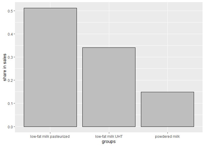 pqcor
pqcor
The function returns Pearson’s correlation coefficient for price and quantity of products with given IDs (defined by the set parameter) and sold in the period. If the set is empty, the function works for all products being available in the period. The figure parameter indicates whether the function returns a figure with a correlation coefficient (TRUE) or just a correlation coefficient (FALSE). For instance:
pqcor(milk, period="2019-05")
#> [1] -0.2047
pqcor(milk, period="2019-05",figure=TRUE)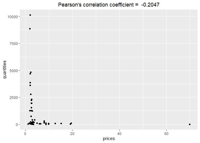 pqcor_fig
The function returns Pearson’s correlation coefficients between price and quantity of products with given IDs (defined by the set parameter) and sold in the time interval defined by the start and end parameters. If the set is empty the function works for all available products. Correlation coefficients are calculated for each month separately. Results are presented in tabular or graphical form depending on the figure parameter. Both cases are presented below:
pqcor_fig(milk, start="2018-12", end="2019-06", figure=FALSE)
#> date correlation
#> 1 2018-12 -0.1835
#> 2 2019-01 -0.1786
#> 3 2019-02 -0.1805
#> 4 2019-03 -0.1956
#> 5 2019-04 -0.1972
#> 6 2019-05 -0.2047
#> 7 2019-06 -0.2037
pqcor_fig(milk, start="2018-12", end="2019-06")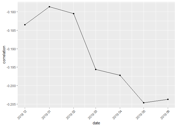 dissimilarity
This function returns a value of the relative price (dSP) and/or quantity (dSQ) dissimilarity measure. In a special case, when the type parameter is set to pq, the function provides the value of dSPQ measure (relative price and quantity dissimilarity measure calculated as min(dSP,dSQ). For instance:
dissimilarity(milk, period1="2018-12",period2="2019-12",type="pq")
#> [1] 0.00004175192
dissimilarity_fig
This function presents values of the relative price and/or quantity dissimilarity measure over time. The user can choose a benchmark period (defined by benchmark) and the type of dissimilarity measure is to be calculated (defined by type). The obtained results of dissimilarities over time can be presented in a dataframe form or via a figure (the default value of figure is TRUE which results a figure). For instance:
dissimilarity_fig(milk, start="2018-12",end="2019-12",type="pq",benchmark="start")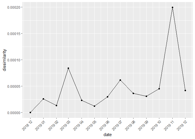 elasticity
This function returns a value of the elasticity of substitution. The procedure of estimation solves the equation: LM(sigma)-CW(sigma)=0 numerically, where LM denotes the Lloyd-Moulton price index, the CW denotes a current weight counterpart of the Lloyd-Moulton price index, and sigma is the elasticity of substitution parameter, which is estimated (see also elasticity2). For example:
elasticity(coffee, start = "2018-12", end = "2019-01")
#> [1] 4.241791
elasticity_fig
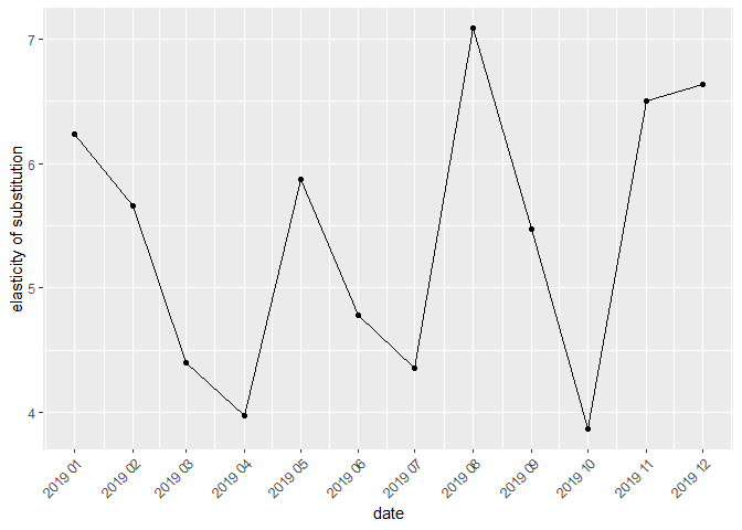
The function provides a data frame or a figure presenting elasticities of substitution calculated for time interval (see the figure parameter). The elasticities of substitution can be calculated for subsequent months or for a fixed base month (see the start parameter) and rest of months from the given time interval (it depends on the fixedbase parameter). The presented function is based on the elasticity function, but see also elasticity2_fig. For instance, to get elasticities of substitution calculated for milk products for subsequent months we run:
elasticity_fig (milk, start = "2018-12", end = "2019-12", fixedbase = FALSE)This package includes 6 functions for calculating the following bilateral unweighted price indices:
| Price Index | Function |
|---|---|
| BMW (2007) | bmw |
| Carli (1804) | carli |
| CSWD (1980,1992) | cswd |
| Dutot (1738) | dutot |
| Jevons (1865) | jevons |
| Harmonic | harmonic |
Each of these functions returns a value (or vector of values) of the choosen unweighted bilateral price index depending on the interval parameter. If the interval parameter is set to TRUE, the function returns a vector of price index values without dates. To get information about both price index values and corresponding dates please see general functions: price_index, price_indices or final_index. None of these functions takes into account aggregating over outlets or product subgroups (to consider these types of aggregating please use the final_index function.) Below are examples of calculations for the Jevons index (in the second case a fixed base month is set to December 2018):
jevons(milk, start="2018-12", end="2020-01")
#> [1] 1.028223
jevons(milk, start="2018-12", end="2020-01", interval=TRUE)
#>  [1] 1.0000000 1.0222661 1.0300191 1.0353857 1.0075504 1.0395393 0.9853148
#> [8] 1.0053100 1.0033727 1.0177604 1.0243906 1.0086291 1.0249373 1.0282234This package includes 26 functions for calculating the following bilateral weighted price indices:
| Price Index | Function |
|---|---|
| AG Mean (2009) | agmean |
| Banajree (1977) | banajree |
| Bialek (2012,2013) | bialek |
| Davies (1924) | davies |
| Drobisch (1871) | drobisch |
| Fisher (1922) | fisher |
| Geary-Khamis (1958,1970) | geary_khamis |
| Geo-Laspeyres | geolaspeyres |
| Geo-Lowe | geolowe |
| Geo-Paasche | geopaasche |
| Geo-Young | geoyoung |
| Geo-hybrid (2020) | geohybrid |
| Hybrid (2020) | hybrid |
| Laspeyres (1871) | laspeyres |
| Lehr (1885) | lehr |
| Lloyd-Moulton (1975,1996) | lloyd_moulton |
| Lowe | lowe |
| Marshall-Edgeworth (1887) | marshall_edgeworth |
| Paasche (1874) | paasche |
| Palgrave (1886) | palgrave |
| Sato-Vartia (1976) | sato_vartia |
| Stuvel (1957) | stuvel |
| Tornqvist (1936) | tornqvist |
| Vartia (1976) | vartia |
| Walsh (1901) | walsh |
| Young | young |
Each of these functions returns a value (or vector of values) of the choosen weighted bilateral price index depending on the interval parameter. If interval parameter is set to TRUE, the function returns a vector of price index values without dates. To get information about both price index values and corresponding dates please see general functions: price_index, price_indices or final_index. None of these functions takes into account aggregating over outlets or product subgroups (to consider these types of aggregating please use the final_index function.) Below are examples of calculations for the Fisher, the Lloyd-Moulton and the Lowe indices (in the last case, the fixed base month is set to December 2019 and the prior period is December 2018):
fisher(milk, start="2018-12", end="2020-01")
#> [1] 0.9615501
lloyd_moulton(milk, start="2018-12", end="2020-01", sigma=0.9)
#> [1] 0.9835069
lowe(milk, start="2019-12", end="2020-02", base="2018-12", interval=TRUE)
#> [1] 1.0000000 0.9880546 1.0024443This package includes 32 functions for calculating the following chain price indices (weighted and unweighted):
| Price Index | Function |
|---|---|
| Chain BMW | chbmw |
| Chain Carli | chcarli |
| Chain CSWD | chcswd |
| Chain Dutot | chdutot |
| Chain Jevons | chjevons |
| Chain Harmonic | chharmonic |
| Chain AG Mean | chagmean |
| Chain Banajree | chbanajree |
| Chain Bialek | chbialek |
| Chain Davies | chdavies |
| Chain Drobisch | chdrobisch |
| Chain Fisher | chfisher |
| Chain Geary-Khamis | chgeary_khamis |
| Chain Geo-Laspeyres | chgeolaspeyres |
| Chain Geo-Lowe | chgeolowe |
| Chain Geo-Paasche | chgeopaasche |
| Chain Geo-Young | chgeoyoung |
| Chain Geo-hybrid | chgeohybrid |
| Chain Hybrid | chhybrid |
| Chain Laspeyres | chlaspeyres |
| Chain Lehr | chlehr |
| Chain Lloyd-Moulton | chlloyd_moulton |
| Chain Lowe | chlowe |
| Chain Marshall-Edgeworth | chmarshall_edgeworth |
| Chain Paasche | chpaasche |
| Chain Palgrave | chpalgrave |
| Chain Sato-Vartia | chsato_vartia |
| Chain Stuvel | chstuvel |
| Chain Tornqvist | chtornqvist |
| Chain Vartia | chvartia |
| Chain Walsh | chwalsh |
| Chain Young | chyoung |
Each time, the interval parameter has a logical value indicating whether the function is to compare the research period defined by end to the base period defined by start (then interval is set to FALSE and it is a default value) or all fixed base indices are to be calculated. In this second case, all months from the time interval <start,end> are considered and start defines the base period (interval is set to TRUE). Here are examples for the Fisher chain index:
chfisher(milk, start="2018-12", end="2020-01")
#> [1] 0.9618094
chfisher(milk, start="2018-12", end="2020-01", interval=TRUE)
#>  [1] 1.0000000 1.0021692 1.0004617 0.9862756 0.9944042 0.9915704 0.9898026
#> [8] 0.9876325 0.9981591 0.9968851 0.9786428 0.9771951 0.9874251 0.9618094This package includes 18 functions for calculating multilateral price indices and one additional and general function (QU) which calculates the quality adjusted unit value index, i.e.:
| Price Index | Function |
|---|---|
| CCDI | ccdi |
| GEKS | geks |
| WGEKS | wgeks |
| GEKS-J | geksj |
| GEKS-W | geksw |
| GEKS-L | geksl |
| WGEKS-L | wgeksl |
| GEKS-GL | geksgl |
| WGEKS-GL | wgeksgl |
| GEKS-AQU | geksaqu |
| WGEKS-AQU | wgeksaqu |
| GEKS-AQI | geksaqi |
| WGEKS-AQI | wgeksaqi |
| GEKS-GAQI | geksgaqi |
| WGEKS-GAQI | wgeksgaqi |
| Geary-Khamis | gk |
| Quality Adjusted Unit Value | QU |
| Time Product Dummy | tpd |
| SPQ | SPQ |
The above-mentioned 18 multilateral formulas (the SPQ index is an exception) consider the time window defined by the wstart and window parameters, where window is a length of the time window (typically multilateral methods are based on a 13-month time window). It measures the price dynamics by comparing the end period to the start period (both start and end must be inside the considered time window). To get information about both price index values and corresponding dates, please see functions: price_index, price_indices or final_index. These functions do not take into account aggregating over outlets or product subgroups (to consider these types of aggregating please use functions: final_index or final_index2). Here are examples for the GEKS formula (see documentation):
geks(milk, start="2019-01", end="2019-04",window=10)
#> [1] 0.9912305
geksl(milk, wstart="2018-12", start="2019-03", end="2019-05")
#> [1] 1.002251
The QU function returns a value of the quality adjusted unit value index (QU index) for the given set of adjustment factors. An additional v parameter is a data frame with adjustment factors for at least all matched prodIDs. It must contain two columns: prodID with unique product IDs and value with corresponding adjustment factors (see documentation). The following example starts from creating a data frame which includes sample adjusted factors:
prodID<-base::unique(milk$prodID)
values<-stats::runif(length(prodID),1,2)
v<-data.frame(prodID,values)
head(v)
#>   prodID   values
#> 1  14215 1.341853
#> 2  14216 1.271927
#> 3  15404 1.742800
#> 4  17034 1.865491
#> 5  34540 1.722126
#> 6  51583 1.194438
and the next step is calculating the QU index which compares December 2019 to December 2018:
QU(milk, start="2018-12", end="2019-12", v)
#> [1] 0.9774024This package includes 17 functions for calculating splice indices:
| Price Index | Function |
|---|---|
| Splice CCDI | ccdi_splcie |
| Splice GEKS | geks_splice |
| Splice weighted GEKS | wgeks_splice |
| Splice GEKS-J | geksj_splice |
| Splice GEKS-W | geksw_splice |
| Splice GEKS-L | geksl_splice |
| Splice weighted GEKS-L | wgeksl_splice |
| Splice GEKS-GL | geksgl_splice |
| Splice weighted GEKS-GL | wgeksgl_splice |
| Splice GEKS-AQU | geksaqu_splice |
| Splice weighted GEKS-AQU | wgeksaqu_splice |
| Splice GEKS-AQI | geksaqi_splice |
| Splice weighted GEKS-AQI | wgeksaqi_splice |
| Splice GEKS-GAQI | geksgaqi_splice |
| Splice weighted GEKS-GAQI | wgeksgaqi_splice |
| Splice Geary-Khamis | gk_splice |
| Splice Time Product Dummy | tpd_splice |
These functions return a value (or values) of the selected multilateral price index extended by using window splicing methods (defined by the splice parameter). Available splicing methods are: movement splice, window splice, half splice, mean splice and their additional variants: window splice on published indices (WISP), half splice on published indices (HASP) and mean splice on published indices (see documentation). The first considered time window is defined by the start and window parameters, where window is a length of the time window (typically multilateral methods are based on a 13-month time window). Functions measure the price dynamics by comparing the end period to the start period, i.e. if the time interval <start, end> exceeds the defined time window then splicing methods are used. If the interval parameter is set to TRUE, then all fixed base multilateral indices are presented (the fixed base month is defined by start). To get information about both price index values and corresponding dates, please see functions: price_index, price_indices or final_index. These functions do not take into account aggregating over outlets or product subgroups (to consider these types of aggregating, please use the final_index function). For instance, let us calculate the extended Time Product Dummy index by using the half splice method with a 10-month time window:
tpd_splice(milk, start="2018-12", end="2020-02",window=10,splice="half",interval=TRUE)
#>  [1] 1.0000000 1.0033636 0.9997753 0.9831710 0.9950045 0.9921984 0.9908530
#>  [8] 0.9861655 0.9994412 0.9945041 0.9805130 0.9813733 0.9889166 0.9628495
#> [15] 1.0021059This package includes 17 functions for calculating extensions of multilateral indices by using the Fixed Base Monthly Expanding Window (FBEW) method:
| Price Index | Function |
|---|---|
| FBEW CCDI | ccdi_fbew |
| FBEW GEKS | geks_fbew |
| FBEW WGEKS | wgeks_fbew |
| FBEW GEKS-J | geksj_fbew |
| FBEW GEKS-W | geksw_fbew |
| FBEW GEKS-L | geksl_fbew |
| FBEW WGEKS-L | wgeksl_fbew |
| FBEW GEKS-GL | geksgl_fbew |
| FBEW WGEKS-GL | wgeksgl_fbew |
| FBEW GEKS-AQU | geksaqu_fbew |
| FBEW WGEKS-AQU | wgeksaqu_fbew |
| FBEW GEKS-AQI | geksaqi_fbew |
| FBEW WGEKS-AQI | wgeksaqi_fbew |
| FBEW GEKS-GAQI | geksgaqi_fbew |
| FBEW WGEKS-GAQI | wgeksgaqi_fbew |
| FBEW Geary-Khamis | gk_fbew |
| FBEW Time Product Dummy | tpd_fbew |
These functions return a value (or values) of the selected multilateral price index extended by using the FBEW method. The FBEW method uses a time window with a fixed base month every year (December). The window is enlarged every month with one month in order to include information from a new month. The full window length (13 months) is reached in December of each year. These functions measure the price dynamics between the end and start periods. A month of the start parameter must be December (see documentation). If the distance between end and start exceeds 13 months, then internal Decembers play a role of chain-linking months. To get information about both price index values and corresponding dates please see functions: price_index, price_indices or final_index. These functions do not take into account aggregating over outlets or product subgroups (to consider these types of aggregating, please use the final_index function). For instance, let us calculate the extended GEKS index by using the FBEW method. Please note that December 2019 is the chain-linking month, i.e.:
geks_fbew(milk, start="2018-12", end="2020-03")
#> [1] 0.9891602
  geks_fbew(milk, start="2018-12", end="2019-12")*
  geks_fbew(milk, start="2019-12", end="2020-03")
#> [1] 0.9891602This package includes 17 functions for calculating extensions of multilateral indices by using the Fixed Base Moving Window (FBMW) method:
| Price Index | Function |
|---|---|
| FBMW CCDI | ccdi_fbmw |
| FBMW GEKS | geks_fbmw |
| FBMW WGEKS | wgeks_fbmw |
| FBMW GEKS-J | geksj_fbmw |
| FBMW GEKS-W | geksw_fbmw |
| FBMW GEKS-L | geksl_fbmw |
| FBMW WGEKS-L | wgeksl_fbmw |
| FBMW GEKS-GL | geksgl_fbmw |
| FBMW WGEKS-GL | wgeksgl_fbmw |
| FBMW GEKS-AQU | geksaqu_fbmw |
| FBMW WGEKS-AQU | wgeksaqu_fbmw |
| FBMW GEKS-AQI | geksaqi_fbmw |
| FBMW WGEKS-AQI | wgeksaqi_fbmw |
| FBMW GEKS-GAQI | geksgaqi_fbmw |
| FBMW WGEKS-GAQI | wgeksgaqi_fbmw |
| FBMW Geary-Khamis | gk_fbmw |
| FBMW Time Product Dummy | tpd_fbmw |
These functions return a value (or values) of the selected multilateral price index extended by using the FBMW method. They measure the price dynamics between the end and start periods and it uses a 13-month time window with a fixed base month taken as year(end)-1. If the distance between end and start exceeds 13 months, then internal Decembers play a role of chain-linking months. A month of the start parameter must be December (see documentation). To get information about both price index values and corresponding dates, please see functions: price_index, price_indices or final_index. These functions do not take into account aggregating over outlets or product subgroups (to consider these types of aggregating, please use the final_index function). For instance, let us calculate the extended CCDI index by using the FBMW method. Please note that December 2019 is the chain-linking month, i.e.:
ccdi_fbmw(milk, start="2018-12", end="2020-03")
#> [1] 0.9874252
    ccdi_fbmw(milk, start="2018-12", end="2019-12")*
    ccdi_fbmw(milk, start="2019-12", end="2020-03")
#> [1] 0.9874252This package includes 3 general functions for price index calculation. The start and end parameters indicate the base and the research period respectively. These function provide value or values (depending on the interval parameter) of the selected price index formula or formulas. If the interval parameter is set to TRUE then it returns a data frame with two columns: dates and index values. Functions price_index and price_indices do not take into account aggregating over outlets or product subgroups and to consider these types of aggregating, please use functions: final_index or final_index2.
price_index
This function returns a value or values of the selected price index. The formula parameter is a character string indicating the price index formula is to be calculated (see documentation). If the selected price index formula needs some additional information it should be defined by additional parameters: window and splice (connected with multilateral indices), base (adequate for the Young and the Lowe indices) or sigma (for the Lloyd-Moulton or the AG mean indices). Sample use:
price_index(milk, start="2019-05", end="2019-06", formula="fisher")
#> [1] 0.9982172
price_index(milk, start="2018-12", end="2020-02",
            formula="tpd_splice",splice="movement",interval=TRUE)
#>       date tpd_splice
#> 1  2018-12  1.0000000
#> 2  2019-01  1.0058281
#> 3  2019-02  1.0008801
#> 4  2019-03  0.9833854
#> 5  2019-04  0.9950913
#> 6  2019-05  0.9915562
#> 7  2019-06  0.9920122
#> 8  2019-07  0.9886072
#> 9  2019-08  0.9998138
#> 10 2019-09  0.9947203
#> 11 2019-10  0.9796047
#> 12 2019-11  0.9784985
#> 13 2019-12  0.9895882
#> 14 2020-01  0.9625456
#> 15 2020-02  1.0031290
price_indices
This is an extended version of the price_index function because it allows us to compare many price index formulas by using one command. The general character of this function mean that, for instance, your one command may calculate two CES indices for two different values of sigma parameter (the elasticity of substitution) or you can select several splice indices and calculate them by using different window lengths and different splicing method. You can control names of columns in the resulting data frame by defining additional parameters: namebilateral, namebindex, namecesindex, namefbmulti, namesplicemulti although their default values correspond to the used price index formulas. Please note that this function is not the most general in the package, i.e. all selected price indices are calculated for the same data set defined by the data parameter and the aggregation over subgroups or outlets are not taken into consideration here (to consider it, please use functions: final_index or final_index2).
For instance, let us use the milk data set and let us calculate the price dynamics for the time interval December 2019 - August 2020) using the following price index formulas: the Fisher index, the Young index with the prior period set to December 2018, the AG mean index with the elasticity of substitution parameter sigma=0.5, the full-window GEKS index with a 9-month window length, the full-window Geary-Khamis index with a 9-month window length, the splice TPD index using a 6-month time window and being extended by using the movement splice method:
price_indices(milk, start="2019-12", end="2020-08", bilateral=c("fisher"),
              bindex=c("young"), base=c("2018-12"),
              cesindex=c("agmean"), sigma=c(0.5),
              fbmulti=c("geks", "gk"), fbwindow=c(9,9),
              splicemulti=c("tpd_splice"),splicewindow=c(6),
              splice=c("movement"), interval=TRUE)
#>      date    fisher     young    agmean      geks        gk tpd_splice
#> 1 2019-12 1.0000000 1.0000000 1.0000000 1.0000000 1.0000000  1.0000000
#> 2 2020-01 0.9740581 0.9892721 0.9940157 0.9751969 0.9695107  0.9734589
#> 3 2020-02 1.0123062 1.0039283 1.0140363 1.0087731 1.0106597  1.0101372
#> 4 2020-03 1.0024357 0.9996556 1.0039500 0.9993375 1.0004861  0.9999263
#> 5 2020-04 0.9779487 0.9896677 0.9972912 0.9752104 0.9710071  0.9771235
#> 6 2020-05 1.0139845 1.0137411 1.0201698 1.0146765 1.0162489  1.0153823
#> 7 2020-06 0.9947352 1.0001336 1.0071368 0.9991796 1.0032921  1.0053941
#> 8 2020-07 1.0033918 1.0041741 1.0090451 1.0063783 1.0077500  1.0098352
#> 9 2020-08 1.0112077 1.0096444 1.0147635 1.0113239 1.0150360  1.0153327
final_index
This function returns a value or values of the selected (final) price index taking into consideration aggregation over product subgroups and/or over outlets (retailer sale points defined in the retID column). If the interval parameter is set to TRUE, then it returns a data frame with two columns: dates and final index values (after optional aggregating). Please note that different index formulas may use different time intervals (or time periods) for calculations and, each time, if the aggrret parameter differs from “none”, aggregation over outlets is done for the set of retIDs being available during all considered months. Moreover, for each outlet, i.e. each retID code, the set of considered prodID codes is limited to those codes which are available simultaneously in all considered months.
Details: the datasets parameter defines the user’s list of data frames with subgroups of sold products (see documentation). The formula parameter is a character string indicating the price index formula is to be calculated (see documentation). If the selected price index formula needs some additional information, it should be defined by additional parameters: window and splice (connected with multilateral indices), base (adequate for the Young and the Lowe indices) or sigma (for the Lloyd-Moulton or the AG mean indices). The aggrret parameter is a character string indicating the formula for aggregation over outlets (retailer sale points defined in the retID column). Available options are: none, laspeyres, paasche, geolaspeyres, geopaasche, fisher, tornqvist, arithmetic and geometric. The first option means that there is no aggregating over outlets. The last two options mean unweighted methods of aggregating, i.e. the arithmetic or the geometric mean is used. Similarly, the aggrsets parameter is a character string indicating the formula for aggregation over product subgroups with identical options as previously.
Example. Let us define two subgroups of milk:
g1<-dplyr::filter(milk, milk$description=="full-fat milk UHT")
g2<-dplyr::filter(milk, milk$description=="low-fat milk UHT")
Now, for the fixed time interval: December 2018 - May 2019, let us calculate the (final) chain Walsh price index (the fixed base month is December 2018) taking into consideration the Laspeyres aggregation over subgroups g1 and g2 and the Fisher aggregation over outlets:
final_index(datasets=list(g1,g2), start="2018-12", end="2019-05",
            formula="chwalsh",
            aggrsets = "laspeyres", aggrret = "fisher",
            interval=TRUE)
#>      date   chwalsh
#> 1 2018-12 1.0000000
#> 2 2019-01 1.0028836
#> 3 2019-02 1.0044375
#> 4 2019-03 1.0088699
#> 5 2019-04 1.0072593
#> 6 2019-05 0.9868345
final_index2
This function returns a value or values of the selected (final) price index taking into consideration aggregation over product subgroups and/or over outlets. Optionally, the function returns a data frame or a figure presenting calculated indices, i.e. the price index for the whole data set and price indices for product subgroups. If the interval parameter is set to TRUE, then it returns a data frame (or a figure) with dates and final index values (after optional aggregating). Please note that different index formulas may use different time intervals (or time periods) for calculations and, each time, if the aggrret parameter differs from “none”, aggregation over outlets is done for the set of retIDs being available during all considered months. Moreover, for each outlet, i.e. each retID code, the set of considered prodID codes is limited to those codes which are available simultaneously in all considered months.
Details: the data parameter defines the user’s data frame with subgroups of sold products (see documentation). The by parameter indicates a grouping variable name, i.e. this column is used for creating subgroups of products. The all parameter is a logical value indicating whether the the selected price index is to be calculated only for the whole set of products or also for created subgroups of products (then all is set to TRUE). The formula parameter is a character string indicating the price index formula is to be calculated (see documentation). If the selected price index formula needs some additional information, it should be defined by additional parameters: window and splice (connected with multilateral indices), base (adequate for the Young and the Lowe indices) or sigma (for the Lloyd-Moulton or the AG mean indices). The aggrret parameter is a character string indicating the formula for aggregation over outlets (retailer sale points defined in the retID column). Available options are: none, laspeyres, paasche, geolaspeyres, geopaasche, fisher, tornqvist, arithmetic and geometric. The first option means that there is no aggregating over outlets. The last two options mean unweighted methods of aggregating, i.e. the arithmetic or the geometric mean is used. Similarly, the aggrsets parameter is a character string indicating the formula for aggregation over product subgroups with identical options as previously. Finally, the figure parameter is a logical value indicating whether the function returns a figure presenting all calculated indices (it works if all and interval are set to TRUE)
Examples. Let us calculate the final Fisher price index (with Laspeyres-type aggregation over subgroups) for the whole data set on coffee and for each product subgroup:
final_index2(data=coffee, by="description",all=TRUE,
             start="2018-12",end="2019-12",
             formula="fisher",
             interval=TRUE,
             aggrsets="laspeyres",aggrret="none",
             figure=FALSE)
#>       date fisher : all groups instant coffee coffee beans ground coffee
#> 1  2018-12           1.0000000      1.0000000    1.0000000     1.0000000
#> 2  2019-01           1.0027599      0.9902984    0.9535798     1.0237694
#> 3  2019-02           1.0115692      0.9753682    1.0992467     1.0144109
#> 4  2019-03           0.9887958      0.9502669    1.0784389     0.9927472
#> 5  2019-04           0.9970437      0.9702892    0.9979700     1.0152654
#> 6  2019-05           1.0108262      0.9421379    1.1001929     1.0356516
#> 7  2019-06           1.0744676      1.0164235    1.0527764     1.1199823
#> 8  2019-07           1.0538767      1.0738491    1.0577020     1.0391339
#> 9  2019-08           1.0379242      1.0225298    1.0998945     1.0329018
#> 10 2019-09           1.0595009      0.9965613    1.0598688     1.1028247
#> 11 2019-10           1.0545770      1.0435102    1.0507304     1.0631821
#> 12 2019-11           0.9879396      0.9683038    1.0094456     0.9960565
#> 13 2019-12           1.0017515      1.0207062    0.9730540     0.9959198
and that can be presented in a figure:
final_index2(data=coffee, by="description",all=TRUE,
             start="2018-12",end="2019-12", formula="fisher",
             interval=TRUE,
             aggrsets="laspeyres",aggrret="none",
             figure=TRUE)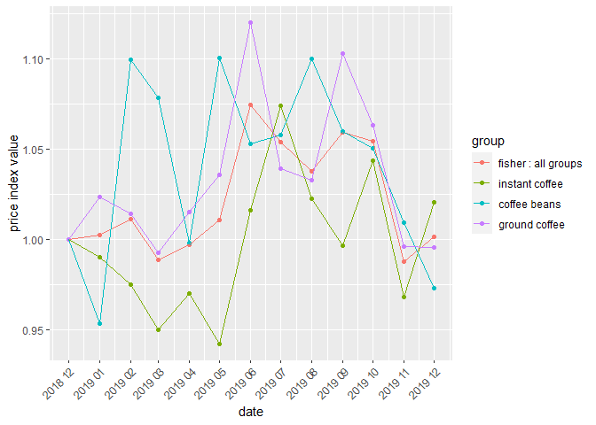
Now, let us calculate and plot the same price index (with no aggregation) for each retID:
final_index2(data=coffee, by="retID",all=TRUE,
             start="2018-12",end="2019-12", formula="fisher",
             interval=TRUE,
             aggrsets="none",aggrret="none",
             figure=TRUE)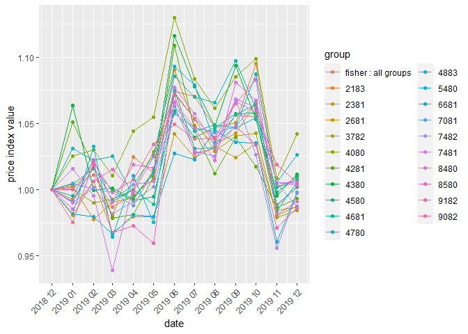
This package includes two functions for a simple graphical comparison of price indices and one function for calculating distances between indices. The first one, i.e. compare_indices, is based on the syntax of the price_indices function and thus it allows us to compare price indices calculated on the same data set. The second function, i.e. compare_final_indices, has a general character since its first argument is a list of data frames which contain results obtained by using the price_index, final_index or final_index2 functions. The third one, i.e. compare_distances, calculates (average) distances between price indices, i.e. the mean absolute distance or root mean square distance is calculated.
compare_indices
This function calculates selected bilateral or/and multilateral price indices and returns a figure with plots of these indices (together with dates on X-axis and a corresponding legend). The function does not take into account aggregating over outlets or product subgroups (to consider these types of aggregating please use functions: final_index and compare_final_indices). Please note that the syntax of the function corresponds to the syntax of the price_indices function (the meaning of parameters is the same - see documentation). For instance, let us compare the price dynamics for the milk dataset for the time interval: December 2018 - December 2019, calculated by using two price index formulas: the chain Jevons index and the full-window GEKS index. The above-mentioned comparison can be made as follows:
compare_indices(milk, start="2018-12",end="2019-12",bilateral=c("chjevons"),
                fbmulti=c("geks"),fbwindow=c(13),
                namebilateral=c("Chain Jevons"), namefbmulti=c("Full GEKS"))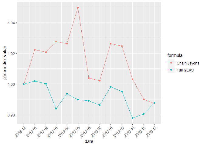
compare_final_indices
This function returns a figure with plots of previously calculated price indices. It allows for graphical comparison of price index values which were previously calculated and now are provided as data frames. To be more precise: the finalindices parameter is a list of data frames with previously calculated price indices. Each data frame must consist of two columns, i.e. the first column must include dates limited to the year and month and the second column must indicate price index values for corresponding dates. The above-mentioned single data frame may be created manually in the previous step or it may be a result of functions: price_index or final_index. All considered data frames must have an identical number of rows. The names parameter is a vector of character strings describing names of presented indices.
For instance, let us compare the impact of the aggregating over outlets on the price index results (e.g. the Fisher formula is the assumed aggregating method). For this purpose, let us calculate the full-window TPD index in two cases: case1 without the above-mentioned aggregation and case2 which considers that aggregation. We use the milk dataset and the yearly time interval:
case1<-price_index(milk, start="2018-12",end="2019-12",
                   formula="tpd", interval=TRUE)
case2<-final_index(datasets=list(milk), start="2018-12", end="2019-12",
                   formula="tpd", aggrsets="none", aggrret = "fisher",
                   interval=TRUE)
The comparison of obtained results can be made as follows (it may be time-consuming on your computer):
compare_final_indices(finalindices=list(case1, case2),names=c("TPD without aggregation","TPD with aggregation"))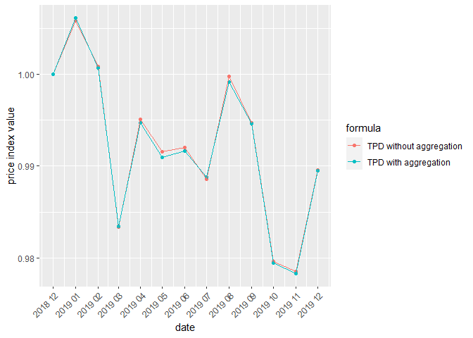
compare_distances
The function calculates average distances between price indices and it returns a data frame with these values for each pair of price indices. The main data parameter is a data frame containing values of indices which are to be compared. The measure parameter specifies what measure should be used to compare the indexes. Possible parameter values are: “MAD” (Mean Absolute Distance) or “RMSD” (Root Mean Square Distance). The results may be presented in percentage points (see the pp parameter) and we can control how many decimal places are to be used in the presentation of results (see the prec parameter).
For instance, let us compare the Jevons, Dutot and Carli indices calculated for the milk data set and for the time interval: December 2018 - December 2019. Let us use the MAD measure for these comparisons:
#Creating a data frame with unweighted bilateral index values
df<-price_indices(milk,
                  bilateral=c("jevons","dutot","carli"),
                  start="2018-12",
                  end="2019-12",
                  interval=TRUE)
#Calculating average distances between indices (in p.p)
compare_distances(df)
#>        jevons dutot carli
#> jevons  0.000 2.482 2.093
#> dutot   2.482 0.000 4.420
#> carli   2.093 4.420 0.000
compare_to_target
The function calculates average distances between considered price indices and the target price index and it returns a data frame with: average distances on the basis of all values of compared indices (distance column), average semi-distances on the basis of values of compared indices which overestimate the target index values (distance_upper column) and average semi-distances on the basis of values of compared indices which underestimate the target index values (distance_lower column).
For instance, let us compare the Jevons, Laspeyres, Paasche and Walsh price indices (calculated for the milk data set and for the time interval: December 2018 - December 2019) with the target Fisher price index:
#Creating a data frame with example bilateral indices
df<-price_indices(milk,
                  bilateral=c("jevons","laspeyres","paasche","walsh"),
                  start="2018-12",end="2019-12",interval=TRUE)
#Calculating the target Fisher price index
target_index<-fisher(milk,start="2018-12",end="2019-12",interval=TRUE)
#Calculating average distances between considered indices and the Fisher index (in p.p)
compare_to_target(df,target=target_index)
#>       index distance distance_lower distance_upper
#> 1    jevons    2.759          0.045          2.714
#> 2 laspeyres    1.429          0.000          1.429
#> 3   paasche    1.403          1.403          0.000
#> 4     walsh    0.174          0.113          0.061