This README file provides an overview of the functionality that can be accomplished with ‘bbsBayes’. It is intended to provide enough information for users to perform, at the very least, replications of status and trend estimates from the Canadian Wildlife Service and/or United States Geological Survey. However, it provides more in-depth and advanced examples for subsetting data, custom regional summaries, and more.
Additional resources: * Introductory bbsBayes Workshop * Journal Article with worked example
bbsBayes is a package to perform hierarchical Bayesian analysis of North American Breeding Bird Survey (BBS) data. ‘bbsBayes’ will run a full model analysis for one or more species that you choose, or you can take more control and specify how the data should be stratified, prepared for JAGS, or modelled.
Option 1: Stable release from CRAN
# To install from CRAN:
install.packages("bbsBayes")
Option 2: Less-stable development version
# To install the development version from GitHub:
install.packages("devtools")
library(devtools)
devtools::install_github("BrandonEdwards/bbsBayes")bbsBayes provides functions for every stage of Breeding Bird Survey data analysis.
You can download BBS data by running fetch_bbs_data.
This will save it to a package-specific directory on your computer. You
must agree to the terms and conditions of the data usage before
downloading. You only need run this function once for each annual update
of the BBS database.
fetch_bbs_data()Stratification plays an important role in trend analysis. Use the
stratify() function for this job. Set the argument
by to stratify by the following options:
bbs_cws – Political region X Bird Conservation region intersection (Canadian Wildlife Service [CWS] method)
bbs_usgs – Political region X Bird Conservation region intersection (United Status Geological Survey [USGS] method)
bcr – Bird Conservation Region only
state – Political Region only
latlong – Degree blocks (1 degree of latitude X 1 degree of longitude)
stratified_data <- stratify(by = "bbs_cws")JAGS models require the data to be sent as a list depending on how
the model is set up. prepare_jags_data subsets the
stratified data based on species and wrangles relevent data to use for
JAGS models.
jags_data <- prepare_jags_data(stratified_data,
                               species_to_run = "Barn Swallow",
                                 min_max_route_years = 5,
                                 model = "gamye",
                                 heavy_tailed = T)
Note: This can take a very long time to run
Once the data has been prepared for JAGS, the model can be run. The
following will run MCMC with default number of iterations. Note that
this step usually takes a long time (e.g., 6-12 hours, or even days
depending on the species, model). If multiple cores are available, the
processing time is reduced with the argument
parallel = TRUE.
mod <- run_model(jags_data = jags_data)Alternatively, you can set how many iterations, burn-in steps, or adapt steps to use, and whether to run chains in parallel
jags_mod <- run_model(jags_data = jags_data,
                               n_saved_steps = 1000,
                               n_burnin = 10000,
                               n_chains = 3,
                               n_thin = 10,
                               parallel = FALSE,
                          parameters_to_save = c("n", "n3", "nu", "B.X", "beta.X", "strata", "sdbeta", "sdX"),
                          modules = NULL)
The run_model function generates a large list (object
jagsUI) that includes the posterior draws, convergence information,
data, etc.
The run_model() function will send a warning if
Gelman-Rubin Rhat cross-chain convergence criterion is > 1.1 for any
of the monitored parameters. Re-running the model with a longer burn-in
and/or more posterior iterations or greater thinning rates may improve
convergence. The seriousness of these convergence failures is something
the user must interpret for themselves. In some cases some parameters of
the model may not be separately estimable, but if there is no direct
inference drawn from those separate parameters, their convergence may
not be necessary. If all or the vast majority of the n parameters have
converged (e.g., you’re receiving this warning message for other
monitored parameters), then inference on population trajectories and
trends from the model are reliable.
jags_mod$n.eff #shows the effective sample size for each monitored parameter
jags_mod$Rhat # shows the Rhat values for each monitored parameter
If important monitored parameters have not converged, we recommend inspecting the model diagnostics with the package ggmcmc.
install.packages("ggmcmc")
S <- ggmcmc::ggs(jags_mod$samples,family = "B.X") #samples object is an mcmc.list object
ggmcmc::ggmcmc(S,family = "B.X") ## this will output a pdf with a series of plots useful for assessing convergence. Be warned this function will be overwhelmed if trying to handle all of the n values from a BBS analysis of a broad-ranged species
Alternatively, the shinystan package has some wonderful interactive tools for better understanding convergence issues with MCMC output.
install.packages("shinystan")
my_sso <- shinystan::launch_shinystan(shinystan::as.shinystan(jags_mod$samples, model_name = "My_tricky_model"))
bbsBayes also includes a function to help re-start an MCMC chain, so that you avoid having to wait for an additional burn-in period.
### if jags_mod has failed to converge...
new_initials <- get_final_values(jags_mod)

jags_mod2 <- run_model(jags_data = jags_data,
                               n_saved_steps = 1000,
                               n_burnin = 0,
                               n_chains = 3,
                               n_thin = 10,
                               parallel = FALSE,
                               inits = new_initials,
                          parameters_to_save = c("n", "n3", "nu", "B.X", "beta.X", "strata", "sdbeta", "sdX"),
modules = NULL)There are a number of tools available to summarize and visualize the posterior predictions from the model. ### Annual Indices of Abundance and Population Trajectories The main monitored parameters are the annual indices of relative abundance within a stratum (i.e., parameters “n[strata,year]”). The time-series of these annual indices form the estimated population trajectories.
indices <- generate_indices(jags_mod = jags_mod,
                            jags_data = jags_data)
By default, this function generates estimates for the continent (i.e., survey-wide) and for the individual strata. However, the user can also select summaries for composite regions (regions made up of collections of strata), such as countries, provinces/states, Bird Conservation Regions, etc. For display, the posterior medians are used for annual indices (instead of the posterior means) due to the asymetrical distributions caused by the log-linear retransformation.
indices <- generate_indices(jags_mod = jags_mod,
                            jags_data = jags_data,
                            regions = c("continental",
                            "national",
                            "prov_state",
                            "stratum"))
                            #also "bcr", "bcr_by_country"
Population trends can be calculated from the series of annual indices of abundance. The trends are expressed as geometric mean rates of change (%/year) between two points in time. \(Trend = (\frac {n[Minyear]}{n[Maxyear]})^{(1/(Maxyear-Minyear))}\)
trends <- generate_trends(indices = indices,
                          Min_year = 1970,
                          Max_year = 2018)
The generate_trends function returns a dataframe with 1
row for each unit of the region-types requested in the
generate_indices function (i.e., 1 for each stratum, 1
continental, etc.). The dataframe has at least 27 columns that report
useful information related to each trend, including the start and end
year of the trend, lists of included strata, total number of routes,
number of strata, mean observed counts, and estimates of the % change in
the population between the start and end years.
The generate_trends function includes some other
arguments that allow the user to adjust the quantiles used to summarize
uncertainty (e.g., interquartile range of the trend estiamtes, or the
67% CIs), as well as include additional calculations, such as the
probability a population has declined (or increased) by > X%.
trends <- generate_trends(indices = indices,
                          Min_year = 1970,
                          Max_year = 2018,
                          prob_decrease = c(0,25,30,50),
prob_increase = c(0,33,100))Generate plots of the population trajectories through time. The
plot_indices() function produces a list of ggplot figures
that can be combined into a single pdf file, or printed to individual
devices.
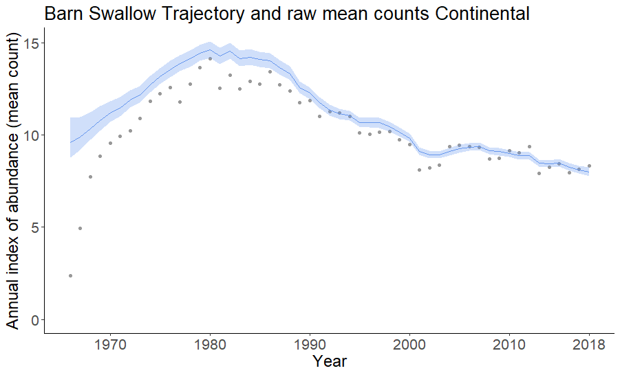
tp = plot_indices(indices = indices,
                         species = "Barn Swallow",
                         add_observed_means = TRUE)
# pdf(file = "Barn Swallow Trajectories.pdf")
# print(tp)
# dev.off()
print(tp[[1]])
print(tp[[2]])  etc.
etc.
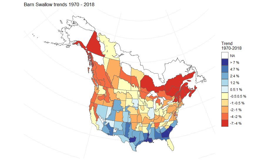
The trends can be mapped to produce strata maps coloured by species population trends.
mp = generate_map(trends,
                  select = TRUE,
                  stratify_by = "bbs_cws",
                  species = "Barn Swallow")
print(mp)
For stratifications that can be compiled by political regions (i.e.,
bbs_cws, bbs_usgs, or state), the
function geofacet_plot will generate a ggplot object that
plots the state and province level population trajectories in facets
arranged in an approximately geographic arrangement. These plots offer a
concise, range-wide summary of a species’ population status and
trends.
  gf <- geofacet_plot(indices_list = indices,
                     select = T,
                     stratify_by = "bbs_cws",
                     multiple = T,
                     trends = trends,
                     slope = F,
                     species = "Barn Swallow")

  #png("BARS_geofacet.png",width = 1500, height = 750,res = 150)
  print(gf)
  #dev.off()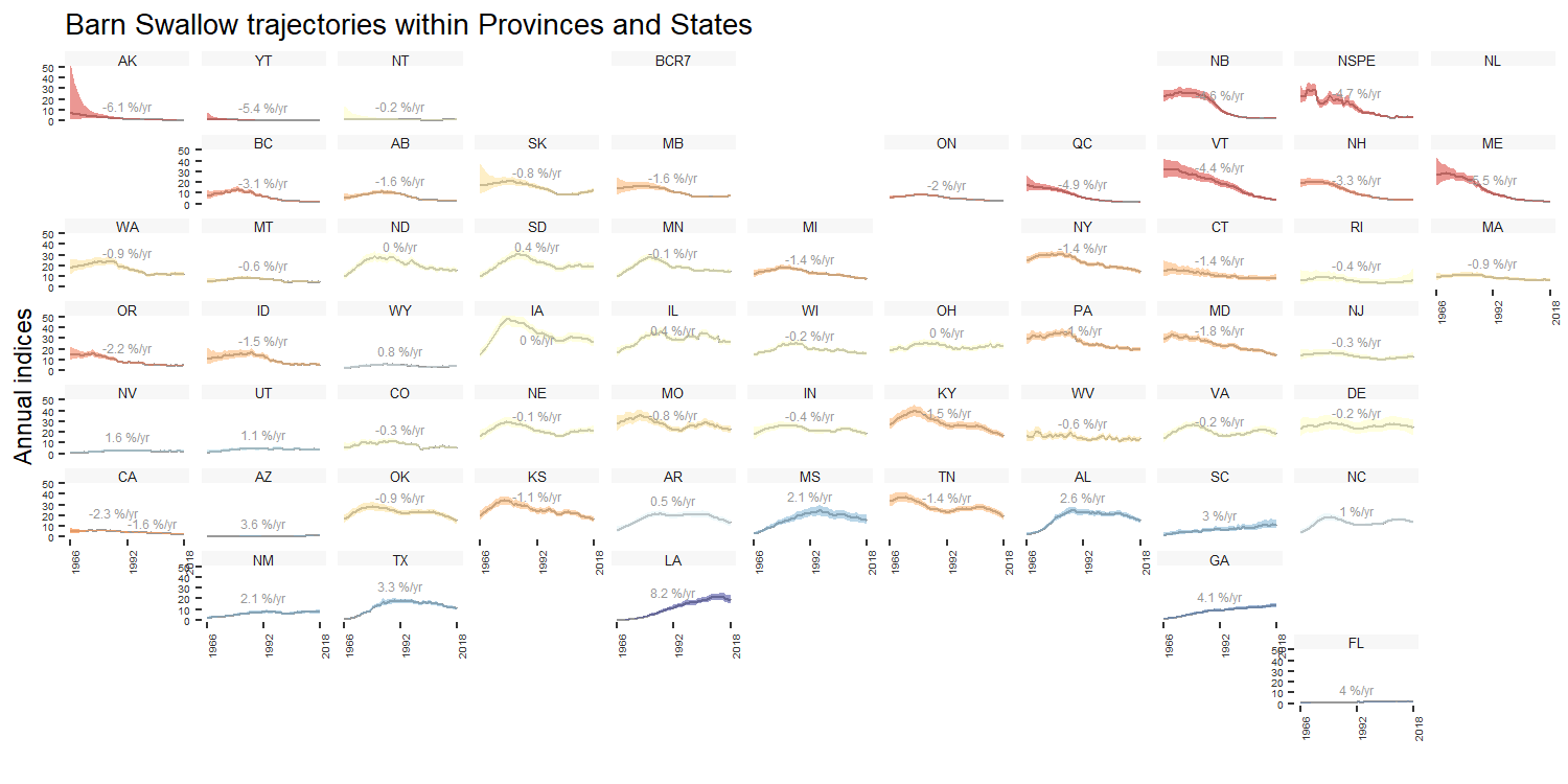
The CWS analysis, as of the 2018 BBS data-version, uses the GAMYE model. It also monitors two estimates of the population trajectory: * one for visualizing the trajectory that includes the annual fluctuations estimated by the year-effects “n” * and another for calculation trends using a trajectory that removes the annual fluctuations around the smooth “n3”.
The full script to run the CWS analysis for the 2018 BBS data version is accessible here: https://github.com/AdamCSmithCWS/BBS_Summaries
species.eng = "Pacific Wren"

stratified_data <- stratify(by = "bbs_cws") #same as USGS but with BCR7 as one stratum and PEI and Nova Scotia combined into one stratum

jags_data <- prepare_jags_data(strat_data = stratified_data,
                                 species_to_run = species.eng,
                                 min_max_route_years = 5,
                                 model = "gamye",
                                 heavy_tailed = T) #heavy-tailed version of gamye model


jags_mod <- run_model(jags_data = jags_data,
                               n_saved_steps = 2000,
                               n_burnin = 10000,
                               n_chains = 3,
                               n_thin = 20,
                               parallel = F,
                          parameters_to_save = c("n","n3","nu","B.X","beta.X","strata","sdbeta","sdX"),
                          modules = NULL)

# n and n3 allow for index and trend calculations, other parameters monitored to help assess convergence and for model testing The USGS analysis, from 2011 through 2017, uses the SLOPE model. Future analyses from the USGS will likely use the first difference model (see, Link et al. 2017 https://doi.org/10.1650/CONDOR-17-1.1)
NOTE: the USGS analysis is not run using the bbsBayes package, and so this analysis may not exactly replicate the published version. However, any variations should be very minor.
species.eng = "Pacific Wren"

stratified_data <- stratify(by = "bbs_usgs") #BCR by province/state/territory intersections

jags_data <- prepare_jags_data(strat_data = stratified_data,
                                 species_to_run = species.eng,
                                 min_max_route_years = 1,
                                 model = "slope",
                                 heavy_tailed = FALSE) #normal-tailed version of slope model


jags_mod <- run_model(jags_data = jags_data,
                               n_saved_steps = 2000,
                               n_burnin = 10000,
                               n_chains = 3,
                               n_thin = 20,
                               parallel = FALSE,
                               track_n = FALSE,
                               parameters_to_save = c("n2"), #more on this alternative annual index below
modules = NULL) The package has (currently) four status and trend models that differ
somewhat in the way they model the time-series of observations. The four
model options are slope, gam, gamye, and firstdiff.
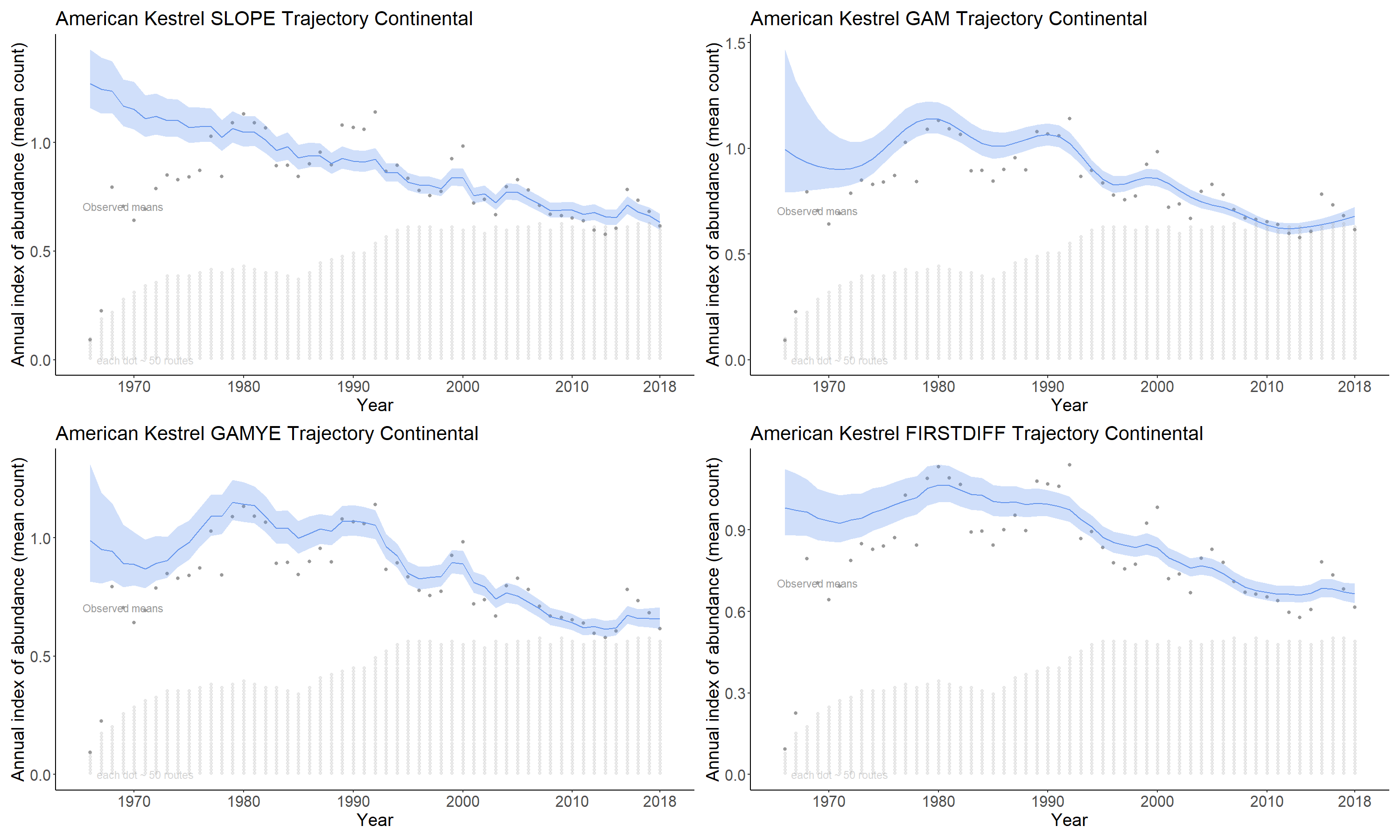
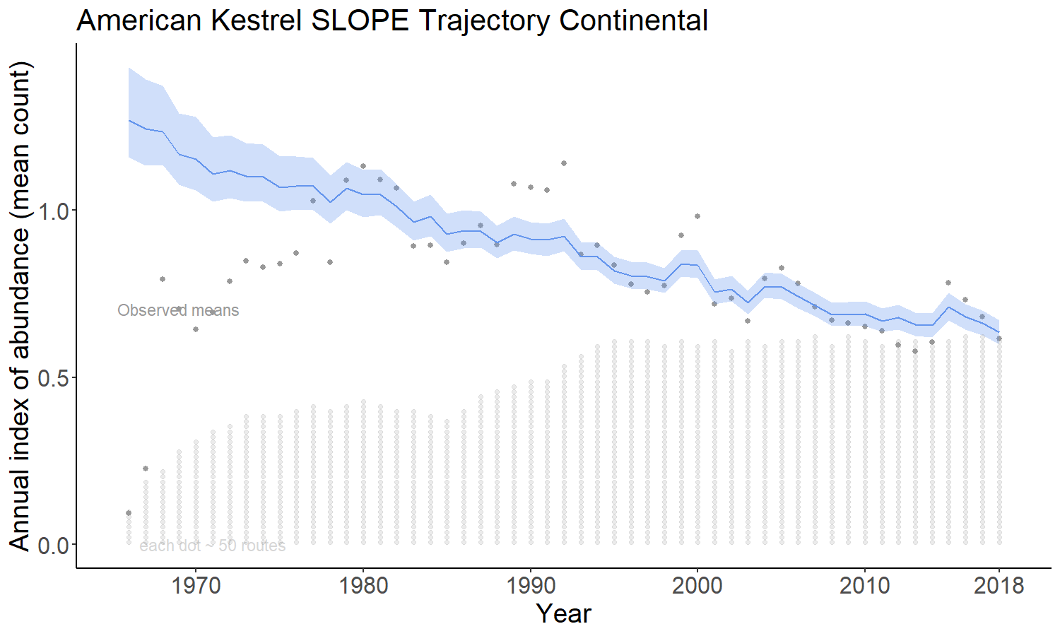
The slope option estimates the time series as a log-linear regression with random year-effect terms that allow the trajectory to depart from the smooth regression line. It is the model used by the USGS and CWS to estimate bbs trends since 2011. The basic model was first described in 2002 (Link and Sauer 2002; https://doi.org/10.1890/0012-9658(2002)083[2832:AHAOPC]2.0.CO;2) and its application to the annual status and trend estimates is documented in Sauer and Link (2011; https://doi.org/10.1525/auk.2010.09220) and Smith et al. (2014; https://doi.org/10.22621/cfn.v128i2.1565).
    #stratified_data <- stratify(by = "bbs_usgs")

    #jags_data_slope <- prepare_jags_data(stratified_data,
    #                           species_to_run = "American Kestrel",
    #                           min_max_route_years = 3,
    #                           model = "slope")

    #jags_mod_full_slope <- run_model(jags_data = jags_data)

    slope_ind <- generate_indices(jags_mod = jags_mod_full_slope,
                                  jags_data = jags_data_slope,
                                  regions = c("continental"))
    slope_plot = plot_indices(indices = slope_ind,
                         species = "American Kestrel SLOPE",
                         add_observed_means = TRUE)
    #png("AMKE_Slope.png", width = 1500,height = 900,res = 150)
    print(slope_plot)
    #dev.off()
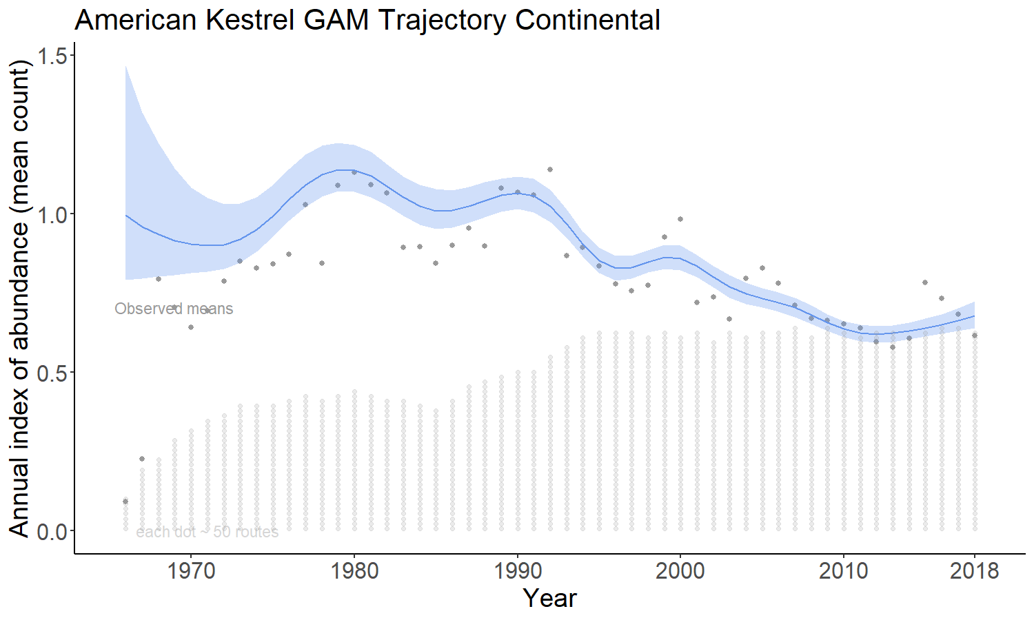
The gam option models the time series as a semiparametric smooth using a Generalized Additive Model (GAM) structure. See https://github.com/AdamCSmithCWS/Smith_Edwards_GAM_BBS for more information (full publication coming soon)
    #stratified_data <- stratify(by = "bbs_usgs")

    #jags_data_gam <- prepare_jags_data(stratified_data,
    #                           species_to_run = "American Kestrel",
    #                           min_max_route_years = 3,
    #                           model = "gam")

    #jags_mod_full_gam <- run_model(jags_data = jags_data)

    gam_ind <- generate_indices(jags_mod = jags_mod_full_gam,
                                jags_data = jags_data_gam,
                                regions = c("continental"))
    gam_plot = plot_indices(indices = gam_ind,
                         species = "American Kestrel GAM",
                         add_observed_means = TRUE)
    #png("AMKE_gam.png", width = 1500,height = 900,res = 150)
    print(gam_plot)
    #dev.off()
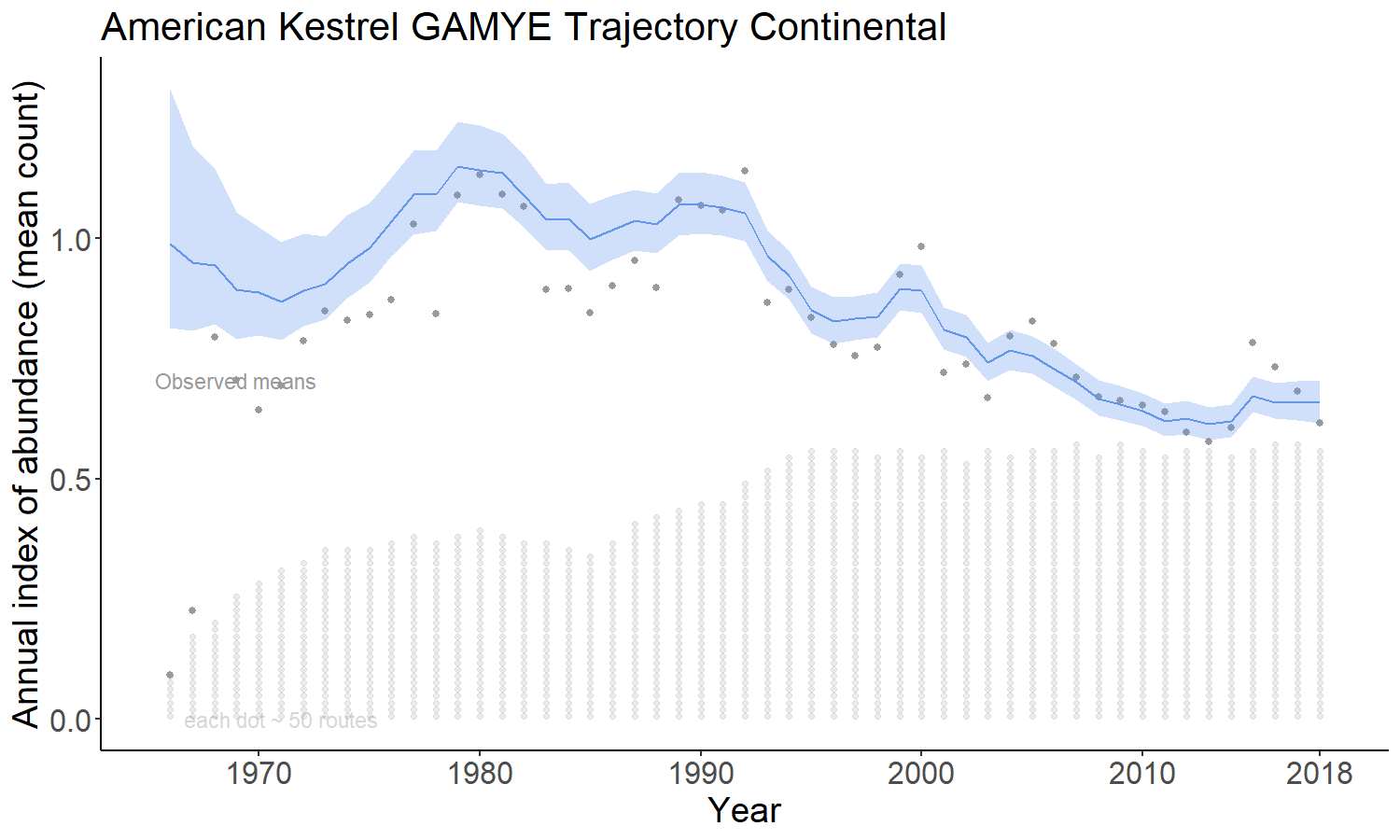
The gamye option includes the semiparametric smooth used in the gam option, but also includes random year-effect terms that track annual fluctuations around the smooth. This is the model that the Canadian Wildlife Service is now using for the annual status and trend estimates.
    #stratified_data <- stratify(by = "bbs_usgs")

    #jags_data_gamye <- prepare_jags_data(stratified_data,
    #                           species_to_run = "American Kestrel",
    #                           min_max_route_years = 3,
    #                           model = "gamye")

    #jags_mod_full_gamye <- run_model(jags_data = jags_data)

    gamye_ind <- generate_indices(jags_mod = jags_mod_full_gamye,
                                  jags_data = jags_data_gamye,
                                  regions = c("continental"))
    gamye_plot = plot_indices(indices = gamye_ind,
                         species = "American Kestrel GAMYE",
                         add_observed_means = TRUE)
    #png("AMKE_gamye.png", width = 1500,height = 900,res = 150)
    print(gamye_plot)
    #dev.off()
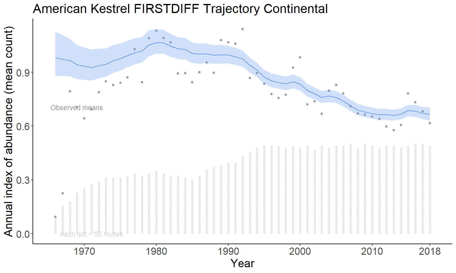
The firstdiff option models the time-series as a random-walk from the first year, so that the first-differences of the sequence of year-effects are random effects with mean = 0 and an estimated variance. This model has been described in Link et al. 2017 https://doi.org/10.1650/CONDOR-17-1.1
    #stratified_data <- stratify(by = "bbs_usgs")

    #jags_data_firstdiff <- prepare_jags_data(stratified_data,
    #                           species_to_run = "American Kestrel",
    #                           min_max_route_years = 3,
    #                           model = "firstdiff")

    #jags_mod_full_firstdiff <- run_model(jags_data = jags_data)

    firstdiff_ind <- generate_indices(jags_mod = jags_mod_full_firstdiff,
                                      jags_data = jags_data_firstdiff,
                                      regions = c("continental"))
    firstdiff_plot = plot_indices(indices = firstdiff_ind,
                         species = "American Kestrel FIRSTDIFF",
                         add_observed_means = TRUE)
    #png("AMKE_firstdiff.png", width = 1500,height = 900,res = 150)
    print(firstdiff_plot)
    #dev.off()
For all of the models, the BBS counts on a given route and year are
modeled as Poisson variables with over-dispersion. The over-dispersion
approach used here is to add a count-level random effect that adds extra
variance to the unit variance:mean ratio of the Poisson. In the
prepare_jags_data function, the user can choose between two
distributions to model the extra-Poisson variance:
heavy_tailed = FALSE)heavy_tailed = TRUE)The heavy-tailed version is well supported for many species, particularly species that are sometimes observed in large groups. Note: the heavy-tailed version can require significantly more time to converge (~2-5 fold increase in processing time).
#stratified_data <- stratify(by = "bbs_usgs")

    #jags_data_firstdiff <- prepare_jags_data(stratified_data,
    #                           species_to_run = "American Kestrel",
    #                           min_max_route_years = 3,
    #                           model = "firstdiff",
    #                           heavy_tailed = TRUE)

#jags_mod_full_firstdiff <- run_model(jags_data = jags_data)In all the models, the default measure of the annual index of
abundance (the yearly component of the population trajectory) is the
derived parameter “n”. The run_model function monitors n by
default, because it is these parameters that form the basis of the
estimated population trajectories and trends.
There are two ways of calculating these annual indices for each
model. The two approaches differ in the way they calculate the
retransformation from the log-scale model parameters to the count-scale
predictions. The user can choose using the following arguments in
run_model() and generate_indices().
mod <- run_model(... ,
                 parameters_to_save = "n",
                 ... )
indices <- generate_indices(... ,
                            alternate_n = "n",
... )parameters_to_save = c("n2"), track_n = FALSE is actually
the standard approach used in the USGS status and trend estimates. It
estimates the the expected count from a new observer-route combination,
assuming the distribution of observer-route effects is approximately
normal. This approach uses a log-normal retransformation factor that
adds half of the estimated variance of observer-route effects to the
log-scale prediction for each year and stratum, then retransforms that
log-scale prediction to the count-scale. This is the approach described
in Sauer and Link (2011; https://doi.org/10.1525/auk.2010.09220).mod <- run_model(... ,
parameters_to_save = "n2",
... )
indices <- generate_indices(... ,
alternate_n = "n2",
... )The default approach parameters_to_save = c("n")
slightly underestimates the uncertainty of the annual indices (slightly
narrower CI width). However, we have chosen this approach as the default
because:
For two of the main model types "slope" and "gamye",
users can choose two different ways to calculate trajectories and
population trends. With these two model types, the population
trajectories are composed of two largely independent components, a
long-term smooth and the random annual fluctuations around that smooth.
Because the two components are largely independent, the population
trajectory can be decomposed.
The default approach is to include the annual fluctuations around the
linear (slope) or GAM-smooth (gamye)
components of the trajectories. These trend estimates are more
comprehensive in that they include the full estimated trajectory, but
they will vary more between subsequent years (e.g., more variability
between a 1970-2017 trend and a 1970-2018 trend), because they include
the effects of the annual fluctuations.
mod <- run_model(... ,
                 parameters_to_save = "n",
                 ... )
indices <- generate_indices(... ,
                            alternate_n = "n",
                            ... )
An alternative approach is to decompose the full trajectory and to
exclude the annual fluctuations around the linear (slope)
or smooth (gamye) components. In this case, the predicted
trends will be much more stable between subsequent years. For the CWS
status and trend analyses, the visualized population trajectories are
calculated using the full trajectory, and the trend estimates are
derived from the decomposed trajectory using only the smooth
component.
mod <- run_model(... ,
parameters_to_save = c("n","n3"),
... )
indices_visualize <- generate_indices(... ,
alternate_n = "n",
... )
indices_trend_calculation <- generate_indices(... ,
alternate_n = "n3",
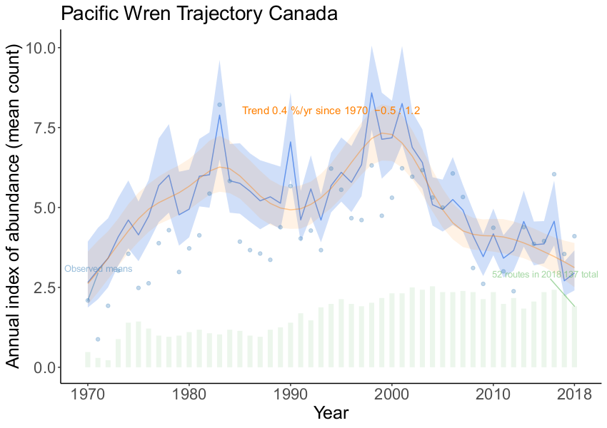
... )For example, the figure below (produced using a modified version of the standard plotting functions), shows the two kinds of trajectories for Pacific Wren from the 2018 CWS analysis. The light-blue trajectory is the visualized trajectory, including the yearly fluctuations. The orange trajectory is the one used for trend calculations, which includes only the GAM-smooth component. For the kinds of broad-scale status assessments that form the primary use of the published estimates of trends, this decomposition is a particularly useful feature of these two models.
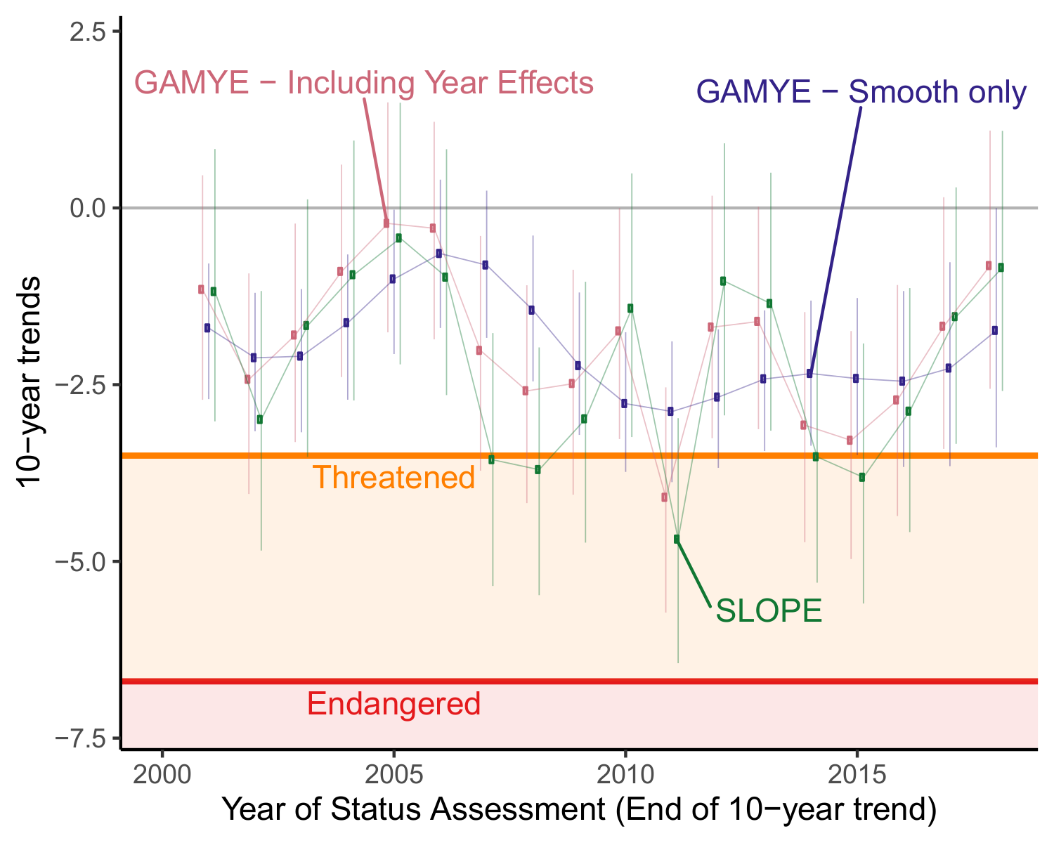
Each point on the graph represents the 10-year trend estimate for Wood Thrush in Canada, ending in a given year (e.g., the points at 2015 represent the species national population trend from 2005-2015). The red and green points are the trend estimates from the default trend estimates derived from the full population trajectories for the gamye and slope models. The Blue points represent the trends calculated using the decomposed trajectory of the gamye model, including only the smooth component. When the annual fluctuations are included (SLOPE and GAMYE including Year Effects), the population trends surpass the IUCN trend-criterion, in some years (e.g., 2011) suggesting that if assessed in those years the species would be listed as Threatened (trend in the orange region). However, a more stable trend estimate from the decomposed trajectory (GAMYE - Smooth only in Blue) shows that the species is probably best thought of as in decline, but not surpassing the Threatened criterion.
The generate_trends() function produces much more than
just the trend estimates.
The default trend calculation is an interval-specific estimate of the geometric mean annual change in the population. \(Trend = (\frac {n[Minyear]}{n[Maxyear]})^{(1/(Maxyear-Minyear))}\) It relies on a comparison of the annual indices in the first and last years of the trend period to quantify the mean rate of population change. However, it ignores the pattern of change between the two end-points.
The user can choose an alternative estimate of change that is
calculated by fitting a log-linear slope to the series of all annual
indices between the two end-points (e.g., all 11 years in a 10-year
trend from 2008-2018). The slope of this line could be expressed as an
average annual percent change across the time-period of interest. If
working with estimates derived from a model with strong annual
fluctuations and for which no decomposition is possible (e.g.,
“firstdiff” model), this slope-based trend may be a more comprehensive
measure of the average population change, that is less dependent on the
particular end-point years. These slope trends can be added to the trend
output table by setting the slope = TRUE argument in
generate_trends(). The standard trends are still
calculated, but additional columns are added that include the alternate
estimates. NOTE: the generate_map() function can map slope
trends as well with the same slope = TRUE argument.
    #jags_data_firstdiff <- prepare_jags_data(stratified_data,
    #                           species_to_run = "American Kestrel",
    #                           model = "firstdiff")

    #jags_mod_full_firstdiff <- run_model(jags_data = jags_data)

    #firstdiff_ind <- generate_indices(jags_mod = jags_mod_full_firstdiff,
    #                                  jags_data = jags_data_firstdiff,
    #                                  regions = c("continental","stratum"))
    fd_slope_trends_08_18 <- generate_trends(indices = firstdiff_ind,
                                             Min_year = 2008,
                                             Max_year = 2018,
                                             slope = TRUE)
    generate_map(fd_slope_trends_0.8_18,
                 slope = TRUE,
                 stratify_by = "bbs_usgs")
)The generate_trends() function also produces estimates
of the overall percent-change in the population between the first and
last years of the trend-period. This calculation is often easier to
interpret than an average annual rate of change. These percent change
estimates have associated uncertainty bounds, and so can be helpful for
deriving statements such as “between 2008 and 2018, the population has
declined by 20 percent, but that estimate is relatively uncertain and
the true decline may be as little as 2 percent or as much as 50
percent”
In addition, the function can optionally calculate the posterior
conditional probability that a population has changed by at least a
certain amount, using the prob_decrease and
prob_increase arguments. These values can be useful for
deriving statements such as “our model suggests that there is a 95%
probability that the species has increased (i.e., > 0% increase) and
a 45 percent probability that the species has increased more than 2-fold
(i.e., > 100% increase)”
    fd_slope_trends_08_18 <- generate_trends(indices = firstdiff_ind,
                                             Min_year = 2008,
                                             Max_year = 2018,
                                             slope = TRUE,
                                             prob_increase = c(0,100))
Yes, you can calculate the trend and trajectories for custom combinations of strata, such as the trends for Eastern and Western populations of Lincoln’s Sparrow.
    #stratification <- "bbs_cws"
    #strat_data <- stratify(by = stratification, sample_data = TRUE)
    #jags_data <- prepare_jags_data(strat_data,
    #                           species_to_run = "Lincoln's Sparrow",
    #                           model = "gamye")

    #jags_mod <- run_model(jags_data = jags_data)
Assuming the above setup has been run. The user could then generate population trajectories using a customized grouping of the original strata.
First extract a dataframe that defines the original strata used in the analysis.
st_comp_regions <- get_composite_regions(strata_type = stratification)The add a column to the dataframe that groups the original strata into the desired custom regions.
st_comp_regions$East_West <- ifelse(st_comp_regions$bcr %in% c(7,8,12:14,22:31),"East","West")st_comp_regions can now be used as the dataframe input to the
argument alt_region_names in generate_indices(), with
“East_West” as the value for the argument regions. The relevant trends
can be calculated using just the generate_trends()
function.
east_west_indices <- generate_indices(jags_mod = jags_mod,
                                      jags_data = jags_data,
                                      alt_region_names = st_comp_regions,
                                      regions = "East_West")
east_west_trends <- generate_trends(indices = east_west_indices)You can easily export any of the bbsBayes models to a text file.
model_to_file(model = "slope",
              filename = "my_slope_model.txt")
Then, you can modify the model text (e.g., try a different prior) and run the modified model
run_model <- function(... ,
                      model_file_path = "my_modified_slope_model.txt",
                      ... )
Details coming soon…
You can even export the bbsBayes model as text, and modify it to add in covariates. For example a GAM smooth to estimate the effect of the day of year on the observations, or an annual weather covariate, or… Then add the relevant covariate data to the jags_data object, and you’re off! We’ll add some more details and examples soon.
Finally, bbsBayes can be used to run Bayesian cross-validations. For
example, the get_final_values() function is useful to
provide an efficient starting point for a cross-validation runs, without
having to wait for another full burn-in period.
Paper that includes an example of how to implement a cross-validation using bbsBayes.
Pre-print: https://doi.org/10.1101/2020.03.26.010215 Supplement: ![]()
NOTE: although bbsBayes includes functions to calculate WAIC, recent work has shown that WAIC performs very poorly with the BBS data (https://doi.org/10.1650/CONDOR-17-1.1). We recommend a k-fold cross-validation approach, as in the above zenodo archive.