![]()
![]()
Accelerate Bayesian analytics workflows in R through interactive modelling, visualization, and inference. Uses probabilistic graphical models as a unifying language for business stakeholders, statisticians, and programmers.
This package relies on the sleek and elegant greta
package for Bayesian inference. greta, in turn, is an
interface into TensorFlow from R. Future iterations of the
causact package will aim to be a front-end into several
universal probablistic programming languages (e.g. Stan, Turing, Gen,
etc.).
Using the causact package for Bayesian inference is
featured in
A Business Analyst's Introduction to Business Analytics
available at https://www.causact.com/.
Feedback and encouragement is appreciated via github issues or Twitter (https://twitter.com/preposterior).
You can install the current release version of the package from CRAN:
install.packages("causact")or the development version from GitHub:
install.packages("remotes")
remotes::install_github("flyaflya/causact")
causact requires the greta package for
Bayesian updating, which in turn, requires a specific version of
TensorFlow. Install both greta and
TensorFlow using the instructions available here: https://www.causact.com/install-tensorflow-greta-and-causact.html.
Example taken from https://www.causact.com/graphical-models-tell-joint-distribution-stories.html#graphical-models-tell-joint-distribution-stories
with the packages dag_foo() functions further described
here:
library(causact)
graph = dag_create() %>%
  dag_node(descr = "Get Card", label = "y",
           rhs = bernoulli(theta),
           data = carModelDF$getCard) %>%
  dag_node(descr = "Card Probability", label = "theta",
           rhs = beta(2,2),
           child = "y") %>%
  dag_plate(descr = "Car Model", label = "x",
            data = carModelDF$carModel,
            nodeLabels = "theta",
            addDataNode = TRUE)
graph %>% dag_render()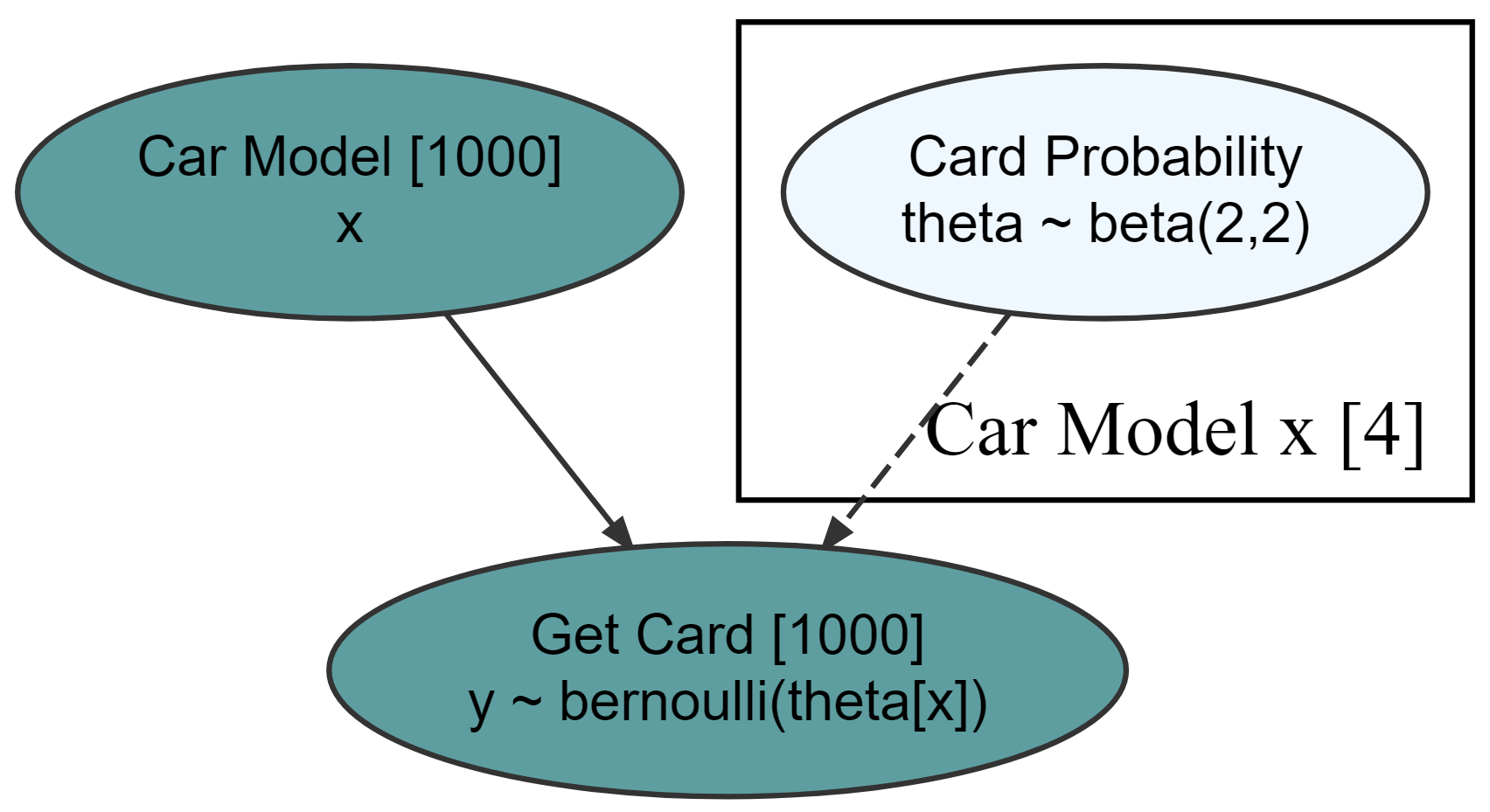
graph %>% dag_render(shortLabel = TRUE)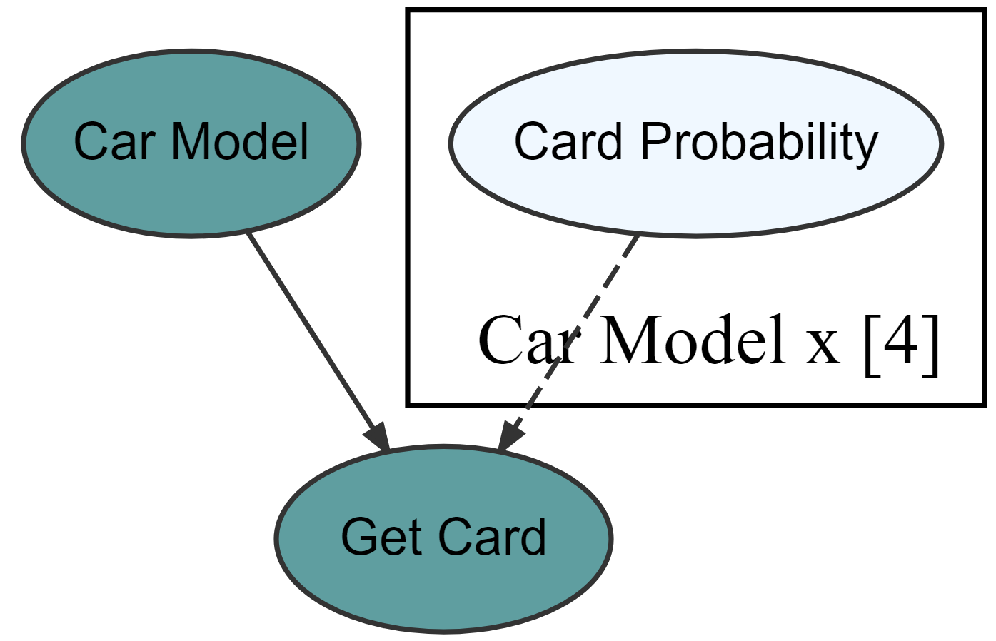
greta code without executing it (for debugging or
learning)library(greta)
#>
#> Attaching package: 'greta'
#> The following objects are masked from 'package:stats':
#>
#> binomial, cov2cor, poisson
#> The following objects are masked from 'package:base':
#>
#> %*%, apply, backsolve, beta, chol2inv, colMeans, colSums, diag,
#> eigen, forwardsolve, gamma, identity, rowMeans, rowSums, sweep,
#> tapply
gretaCode = graph %>% dag_greta(mcmc = FALSE)
#> ## The below greta code will return a posterior distribution
#> ## for the given DAG. Either copy and paste this code to use greta
#> ## directly, evaluate the output object using 'eval', or
#> ## or (preferably) use dag_greta(mcmc=TRUE) to return a data frame of
#> ## the posterior distribution:
#> y <- as_data(carModelDF$getCard) #DATA
#> x <- as.factor(carModelDF$carModel) #DIM
#> x_dim <- length(unique(x)) #DIM
#> theta <- beta(shape1 = 2, shape2 = 2, dim = x_dim) #PRIOR
#> distribution(y) <- bernoulli(prob = theta[x]) #LIKELIHOOD
#> gretaModel <- model(theta) #MODEL
#> meaningfulLabels(graph)
#> draws <- mcmc(gretaModel) #POSTERIOR
#> drawsDF <- replaceLabels(draws) %>% as.matrix() %>%
#> dplyr::as_tibble() #POSTERIOR
#> tidyDrawsDF <- drawsDF %>% addPriorGroups() #POSTERIORgreta
codelibrary(greta)
drawsDF = graph %>% dag_greta()
drawsDF ### see top of data frame
#> # A tibble: 4,000 x 4
#> theta_JpWrnglr theta_KiaForte theta_SbrOtbck theta_ToytCrll
#> <dbl> <dbl> <dbl> <dbl>
#> 1 0.878 0.219 0.560 0.211
#> 2 0.839 0.296 0.660 0.227
#> 3 0.840 0.229 0.571 0.209
#> 4 0.864 0.175 0.669 0.199
#> 5 0.809 0.307 0.537 0.204
#> 6 0.823 0.269 0.593 0.203
#> 7 0.865 0.178 0.644 0.204
#> 8 0.879 0.274 0.555 0.197
#> 9 0.849 0.189 0.623 0.230
#> 10 0.817 0.231 0.577 0.180
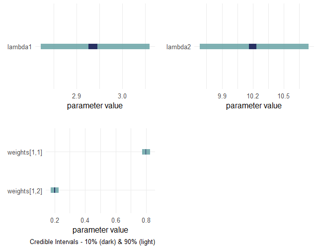
#> # ... with 3,990 more rowsdrawsDF %>% dagp_plot()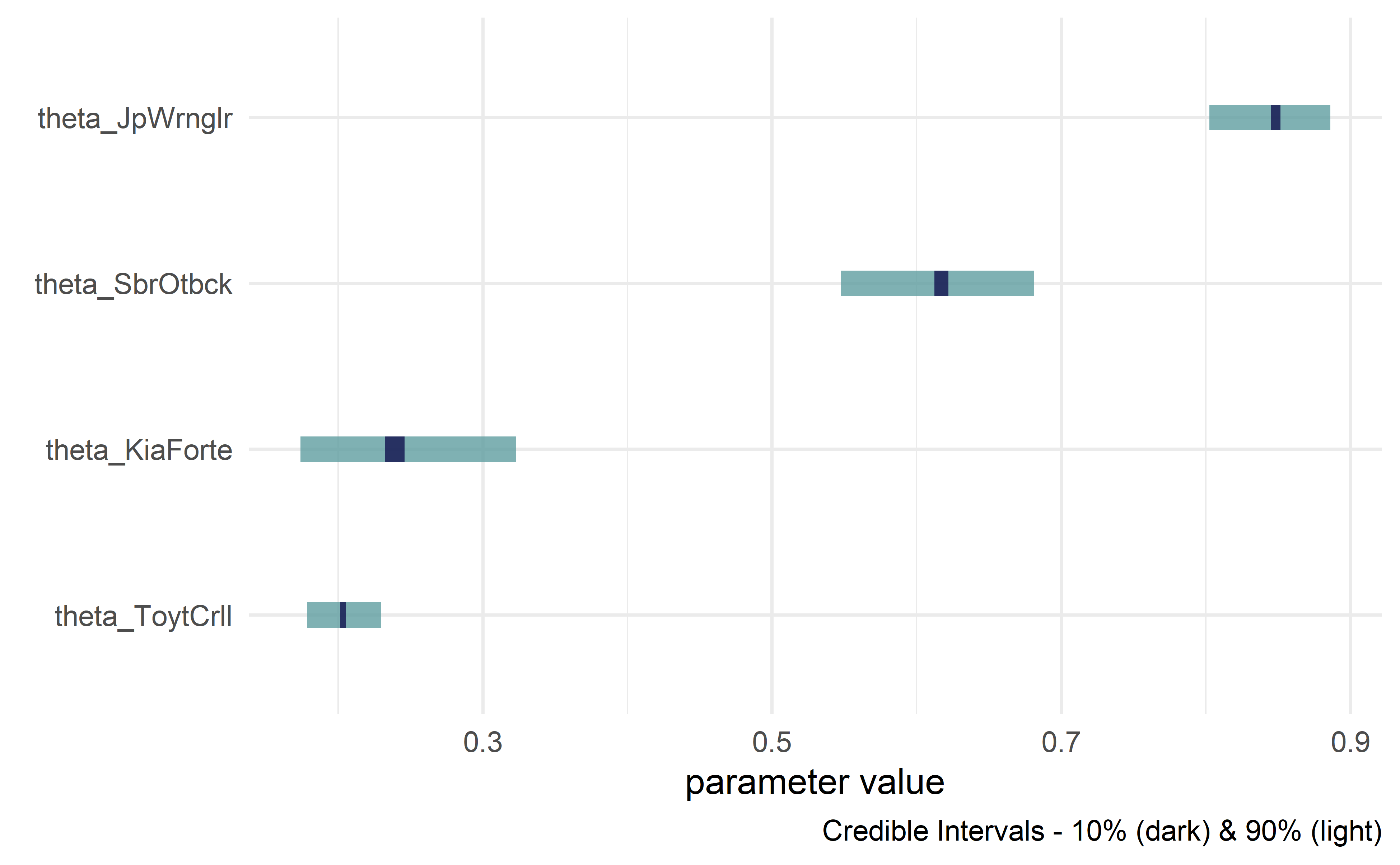
Credible interval plots.
Whether you encounter a clear bug, have a suggestion for improvement,
or just have a question, we are thrilled to help you out. In all cases,
please file a GitHub issue. If
reporting a bug, please include a minimal reproducible example. If
encountering issues installing greta, please seek help at
the greta discussion
forum.
We welcome help turning causact into the most intuitive
and fastest method of converting stakeholder narratives about
data-generating processes into actionable insight from posterior
distributions. If you want to help us achieve this vision, we welcome
your contributions after reading the new
contributor guide. Please note that this project is released with a
Contributor
Code of Conduct. By participating in this project you agree to abide
by its terms.
For more info, see
A Business Analyst's Introduction to Business Analytics
available at https://www.causact.com. You can also check out the
package’s vignette:
vignette("narrative-to-insight-with-causact"). Two
additional examples are shown below.
McElreath, Richard. Statistical rethinking: A Bayesian course with examples in R and Stan. Chapman and Hall/CRC, 2018.
library(greta)
library(tidyverse)
library(causact)

# data object used below, chimpanzeesDF, is built-in to causact package

graph = dag_create() %>%
  dag_node("Pull Left Handle","L",
           rhs = bernoulli(p),
           data = causact::chimpanzeesDF$pulled_left) %>%
  dag_node("Probability of Pull", "p",
           rhs = ilogit(alpha + gamma + beta),
           child = "L") %>%
  dag_node("Actor Intercept","alpha",
           rhs = normal(alphaBar, sigma_alpha),
           child = "p") %>%
  dag_node("Block Intercept","gamma",
           rhs = normal(0,sigma_gamma),
           child = "p") %>%
  dag_node("Treatment Intercept","beta",
           rhs = normal(0,0.5),
           child = "p") %>%
  dag_node("Actor Population Intercept","alphaBar",
           rhs = normal(0,1.5),
           child = "alpha") %>%
  dag_node("Actor Variation","sigma_alpha",
           rhs = exponential(1),
           child = "alpha") %>%
  dag_node("Block Variation","sigma_gamma",
           rhs = exponential(1),
           child = "gamma") %>%
  dag_plate("Observation","i",
            nodeLabels = c("L","p")) %>%
  dag_plate("Actor","act",
            nodeLabels = c("alpha"),
            data = chimpanzeesDF$actor,
            addDataNode = TRUE) %>%
  dag_plate("Block","blk",
            nodeLabels = c("gamma"),
            data = chimpanzeesDF$block,
            addDataNode = TRUE) %>%
  dag_plate("Treatment","trtmt",
            nodeLabels = c("beta"),
            data = chimpanzeesDF$treatment,
addDataNode = TRUE)graph %>% dag_render(width = 2000, height = 800)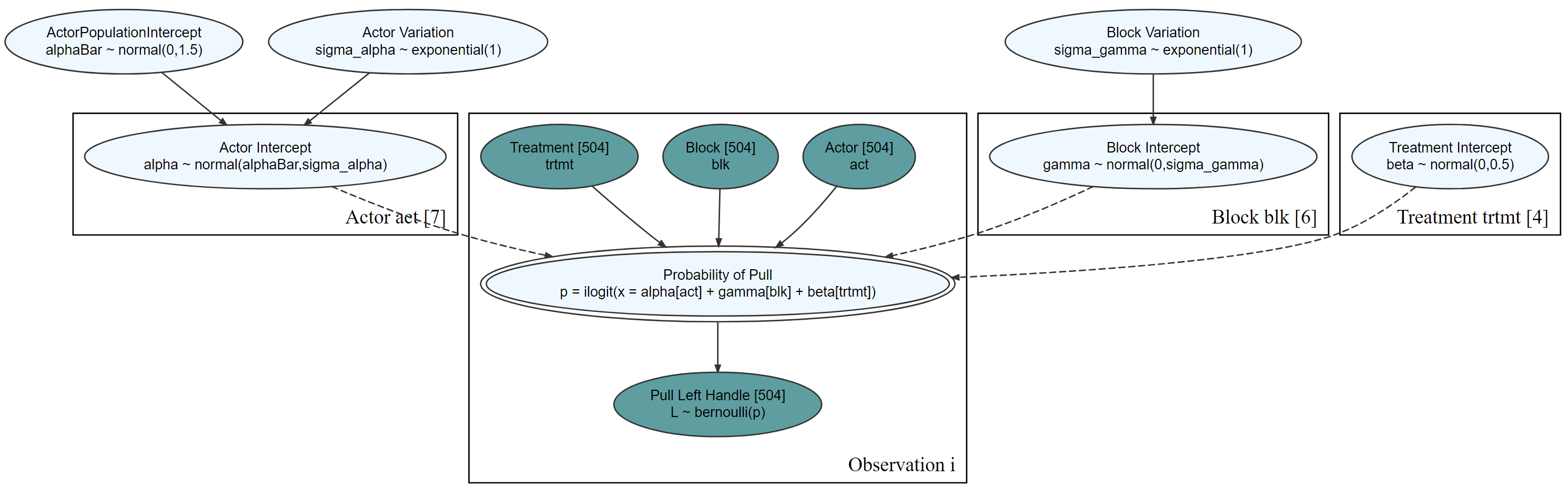
graph %>% dag_render(shortLabel = TRUE)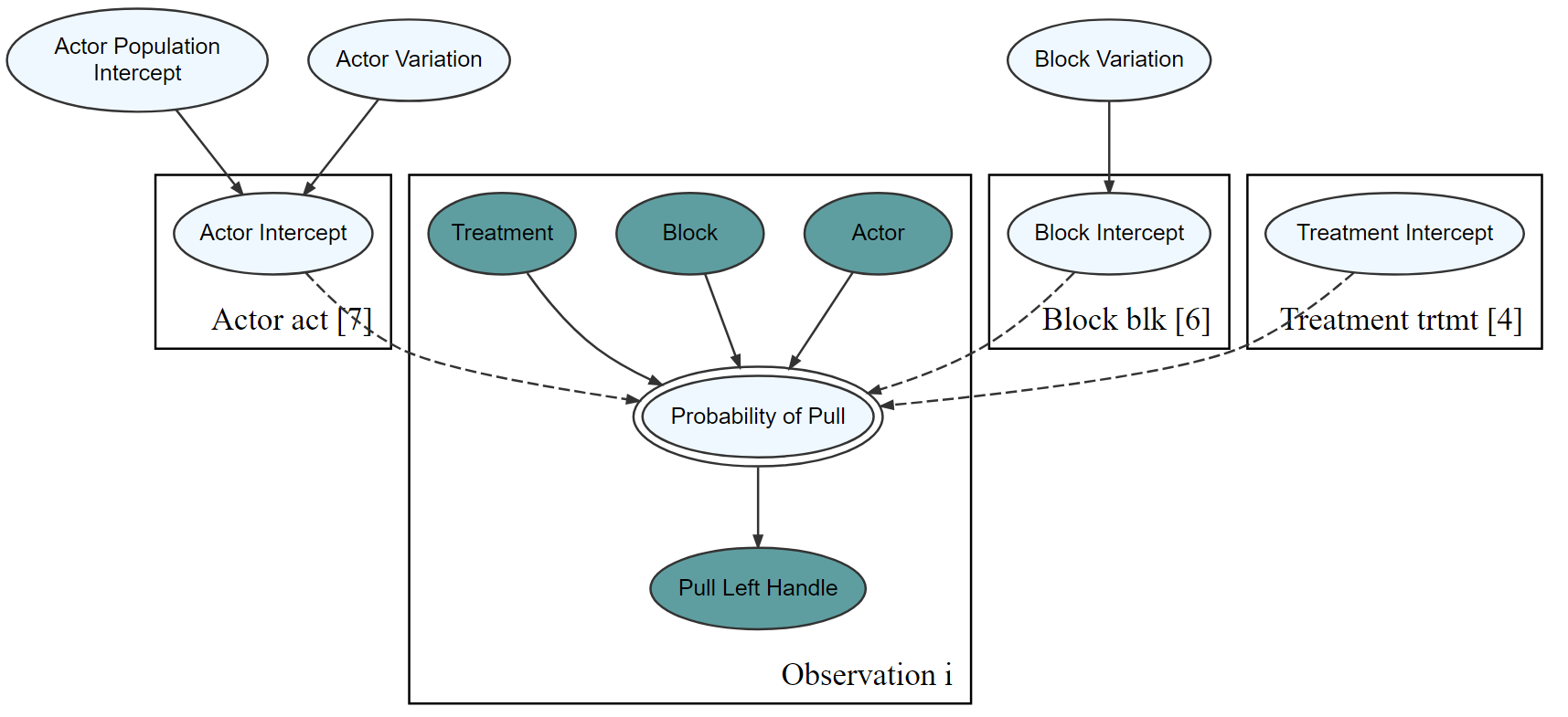
drawsDF = graph %>% dag_greta()drawsDF %>% dagp_plot()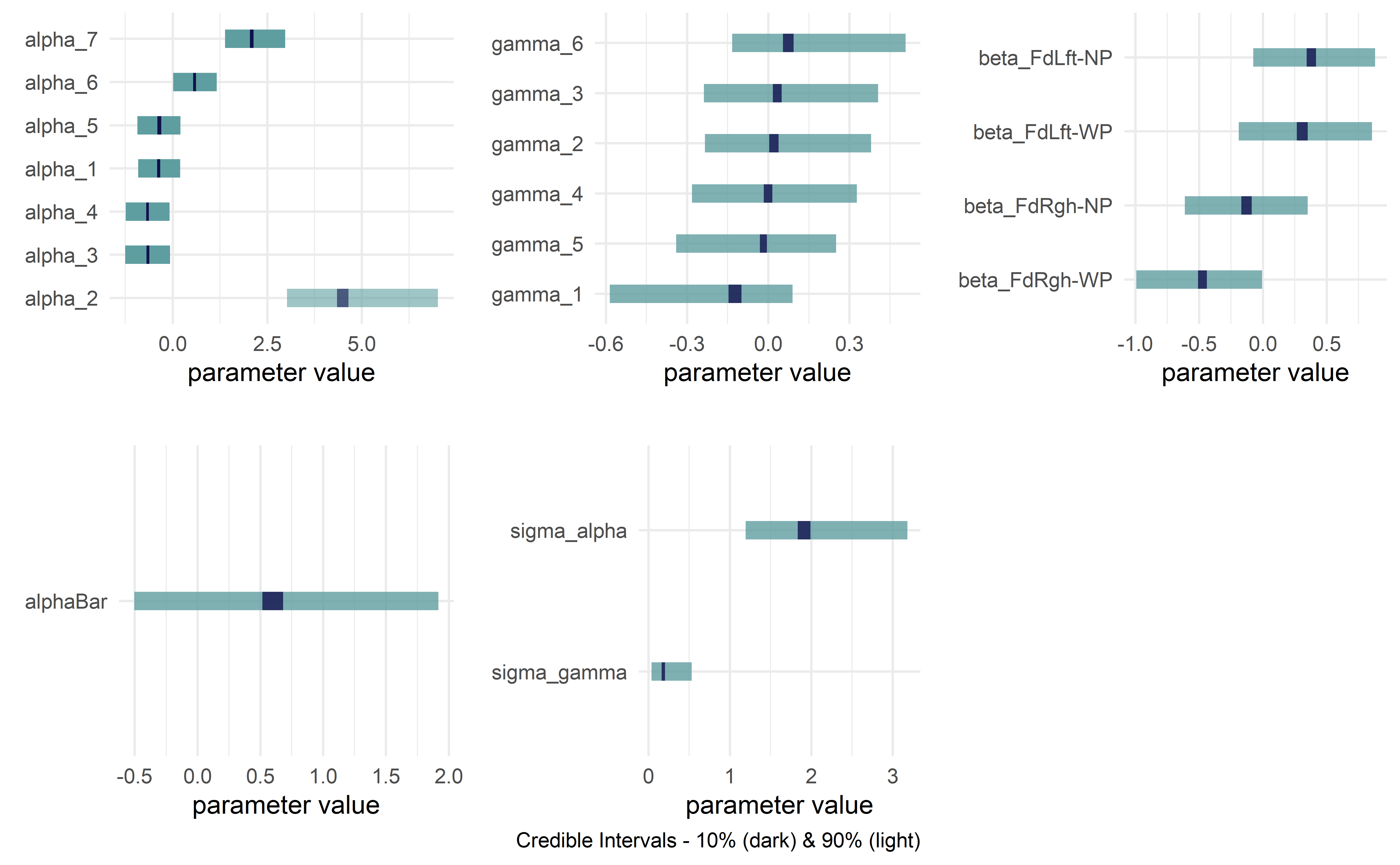
Gelman, Andrew, Hal S. Stern, John B. Carlin, David B. Dunson, Aki Vehtari, and Donald B. Rubin. Bayesian data analysis. Chapman and Hall/CRC, 2013.
library(greta)
library(tidyverse)
library(causact)

# data object used below, schoolDF, is built-in to causact package

graph = dag_create() %>%
  dag_node("Treatment Effect","y",
           rhs = normal(theta, sigma),
           data = causact::schoolsDF$y) %>%
  dag_node("Std Error of Effect Estimates","sigma",
           data = causact::schoolsDF$sigma,
           child = "y") %>%
  dag_node("Exp. Treatment Effect","theta",
           child = "y",
           rhs = avgEffect + schoolEffect) %>%
  dag_node("Pop Treatment Effect","avgEffect",
           child = "theta",
           rhs = normal(0,30)) %>%
  dag_node("School Level Effects","schoolEffect",
           rhs = normal(0,30),
           child = "theta") %>%
  dag_plate("Observation","i",nodeLabels = c("sigma","y","theta")) %>%
  dag_plate("School Name","school",
            nodeLabels = "schoolEffect",
            data = causact::schoolsDF$schoolName,
addDataNode = TRUE)graph %>% dag_render()
drawsDF = graph %>% dag_greta()drawsDF %>% dagp_plot()
#### use dirichlet instead
library(greta)
library(tidyverse)
library(causact)

## sample data - try to recover params
x <- c(rpois(800, 3),rpois(200, 10))

graph = dag_create() %>%  ## create generative DAG
  dag_node("Mixed Var","x",
           rhs = mixture(alpha,beta,
                         weights = t(weights)),
           data = x) %>%
  dag_node("Count Var 1","alpha",
           rhs = poisson(lambda1),
           child = "x") %>%
  dag_node("Count Var 2","beta",
           rhs = poisson(lambda2),
           child = "x") %>%
  dag_node("Weight Vars","weights",
           rhs = dirichlet(t(c(1,1))),
           child = "x") %>%
  dag_node("Exp Rate 1","lambda1",
           rhs = uniform(1,5),
           child = "alpha") %>%
  dag_node("Exp Rate 2","lambda2",
           rhs = uniform(6,20),
child = "beta")graph %>% dag_render()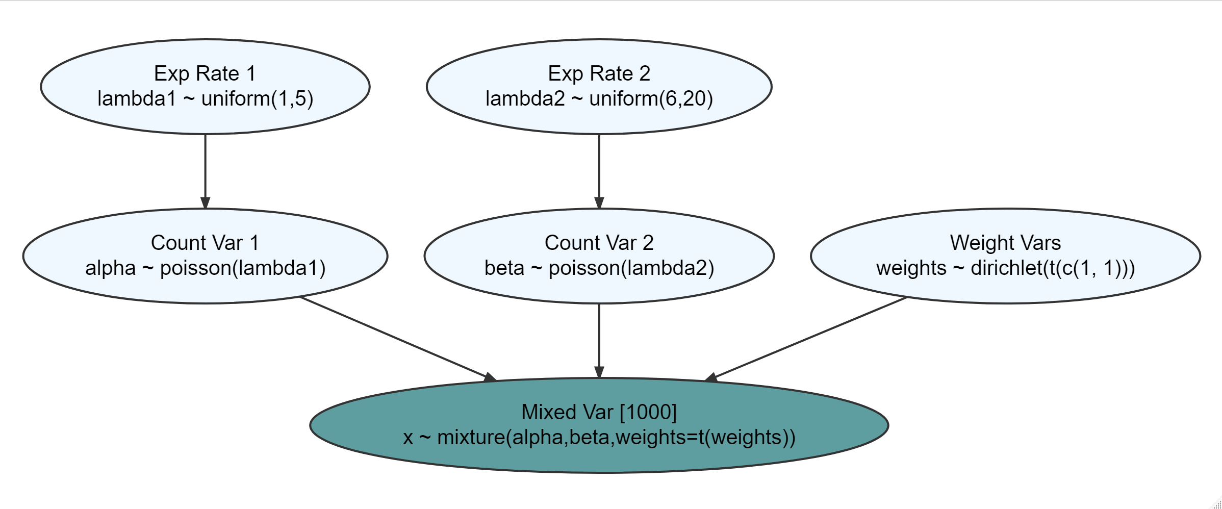
drawsDF %>% dagp_plot()