

The goal of crestr is to enable probabilistic
reconstructions of past climate change from fossil assemblage data. The
approach is based on the estimation of conditional responses of
different bio-proxies to various climate parameters. These responses
take the form of probability density functions (PDFs). The
details of the method have been described in Chevalier et
al. (2014), the calibrated data are presented in Chevalier
(2019) and the package is fully described in Chevalier
(2022).
You can install the package from CRAN.
install.packages("crestr")You can also install the development version from GitHub with:
if(!require(devtools)) install.packages("devtools")
devtools::install_github("mchevalier2/crestr")
NOTE: If the install fails, it is possible that gdal or PROJ are not installed on your system. Ample documentation exists online to guide you through the installation of these two elements to your own system.
If you experience any trouble while using this package, or if you think of additional functionalities to incorporate to the package, please contact me at chevalier.manuel@gmail.com or open a discussion here.
crestrThe package is fully documented and the help of each function can be
accessed with ?function. More detailed information as well
as documented examples are available from https://mchevalier2.github.io/crestr/.
The following example illustrates the basics of crestr
using pseudo-data (i.e. randomly generated data).
library(crestr)
## loading example data
data(crest_ex)
data(crest_ex_pse)
data(crest_ex_selection)
Let’s first have a look at the data. The dataset is composed of 20 fossil samples from which 7 taxa have been identified. The data are expressed in percentages.
## the first 6 samples
head(crest_ex)
#>          Age Taxon1 Taxon2 Taxon3 Taxon4 Taxon5 Taxon6 Taxon7
#> Sample_1   1      0      0     45      1     22     32      1
#> Sample_2   2      0      0     50      0     23     27      0
#> Sample_3   3      0      0     49      0     25     26      0
#> Sample_4   4      0      0     37      0     27     36      0
#> Sample_5   5      0      3     36      3     18     40      0
#> Sample_6   6      2      2     25      0     21     50      0
##
## the structure of the data frame
str(crest_ex)
#> 'data.frame':    20 obs. of  8 variables:
#>  $ Age   : int  1 2 3 4 5 6 7 8 9 10 ...
#>  $ Taxon1: int  0 0 0 0 0 2 3 5 10 15 ...
#>  $ Taxon2: int  0 0 0 0 3 2 5 5 12 8 ...
#>  $ Taxon3: int  45 50 49 37 36 25 18 17 10 12 ...
#>  $ Taxon4: int  1 0 0 0 3 0 0 6 15 14 ...
#>  $ Taxon5: int  22 23 25 27 18 21 21 20 16 13 ...
#>  $ Taxon6: int  32 27 26 36 40 50 53 47 37 38 ...
#>  $ Taxon7: int  1 0 0 0 0 0 0 0 0 0 ...
For each reconstruction, a proxy-species equivalency (‘pse’) table must be provided. Here, with the 7 pseudo-taxa, it looks like:
crest_ex_pse
#>   Level      Family    Genus Species ProxyName
#> 1     3 Randomaceae Randomus  Taxon1    Taxon1
#> 2     3 Randomaceae Randomus  Taxon2    Taxon2
#> 3     3 Randomaceae Randomus  Taxon3    Taxon3
#> 4     3 Randomaceae Randomus  Taxon4    Taxon4
#> 5     3 Randomaceae Randomus  Taxon5    Taxon5
#> 6     3 Randomaceae Randomus  Taxon6    Taxon6
#> 7     3 Randomaceae Randomus  Taxon7    Taxon7
Finally, unique sets of taxa can be specified to reconstruct each climate variable. In the example, bio1 (mean annual temperature) and bio12 (annual precipitation) will be reconstructed. The dataset has been designed so that Taxa 1, 2, 3 and 7 are sensitive to bio1 while Taxa 1, 4, 5 and 7 are sensitive to bio12. Check https://mchevalier2.github.io/crestr/articles/get-started.html for more details on this selection.
crest_ex_selection
#>        bio1 bio12
#> Taxon1    1     1
#> Taxon2    1     0
#> Taxon3    1     0
#> Taxon4    0     1
#> Taxon5    0     1
#> Taxon6    0     0
#> Taxon7    1     1
These pseudo-data can be provided to the crest function and provided some parameters (see the full vignettes for a detail of these parameters), the reconstructions will be processed.
recons <- crest(
   df = crest_ex, pse = crest_ex_pse, taxaType = 0,
   climate = c("bio1", "bio12"), bin_width = c(2, 50),
   shape = c("normal", "lognormal"),
   selectedTaxa = crest_ex_selection, dbname = "crest_example"
)
#> Warning in crest.get_modern_data(pse = pse, taxaType = taxaType, climate
#> = climate, : The classification of one or more taxa into species was not
#> successful. Check `x$misc$taxa_notes` for details.
A specific print function was created to summarise the crestObj.
recons
#> *
#> * Summary of the crestObj named ``:
#> *   x Calibration data formatted .. TRUE
#> *   x PDFs fitted ................. TRUE
#> *   x Climate reconstructed ....... TRUE
#> *   x Leave-One-Out analysis ...... FALSE
#> *
#> * The dataset to be reconstructed (`df`) is composed of 20 samples with 7 taxa.
#> * Variables to analyse: bio1, bio12
#> *
#> * The calibration dataset was defined using the following set of parameters:
#> *   x Proxy type ............ Example dataset
#> *   x Longitude ............. [0 - 15]
#> *   x Latitude .............. [0 - 15]
#> *
#> * The PDFs were fitted using the following set of parameters:
#> *   x Minimum distinct of distinct occurences .. 20
#> *   x Weighted occurence data .................. FALSE
#> *   x Number of points to fit the PDFs ......... 500
#> *   x Geographical weighting ................... TRUE
#> *       Using bins of width .................... bio1: 2
#> *       ________________________________________ bio12: 50
#> *   x Weighting of the climate space ........... TRUE
#> *   x Shape of the PDFs ........................ bio1: normal
#> *     __________________________________________ bio12: lognormal
#> *
#> * Of the 7 taxa provided in `df` and `PSE`, 1 cannot be analysed.
#> * (This may be expected, but check `$misc$taxa_notes` for additional details.)
#> *
#> * The reconstructions were performed with the following set of parameters:
#> *   x Minimum presence value .................. 0
#> *   x Weighting of the taxa ................... normalisation
#> *   x Calculated uncertainties ................ 0.5, 0.95
#> *   x Number of taxa selected to reconstruct .. bio1: 3
#> *     ----------------------------------------- bio12: 3
#> *
The climate sampled by the data can be graphically represented for a quick assessment of the calibration dataset.
plot_climateSpace(recons)
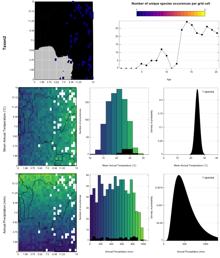
Additional graphical tools can be used to assess which taxa should/could be used for each variable. On the following example, it is clear that Taxon2 has a much stronger correlation with bio1 than to bio12, hence its selection for bio1 only.
plot_taxaCharacteristics(recons, taxanames='Taxon2')
The results can be quickly visualised using the plot function and the
reconstructed climate values can be accessed from the nested
recons object:
names(recons)
#> [1] "inputs"          "parameters"      "modelling"       "reconstructions"
#> [5] "misc"
lapply(recons$reconstructions, names)
#> $bio1
#> [1] "likelihood"    "uncertainties" "optima"
#>
#> $bio12
#> [1] "likelihood" "uncertainties" "optima"head(recons$reconstructions$bio1$optima)
#> Age optima mean
#> 1 1 15.71142 15.69949
#> 2 2 15.71142 15.69949
#> 3 3 15.71142 15.69949
#> 4 4 15.71142 15.69949
#> 5 5 17.31463 17.29054
#> 6 6 18.11623 18.12464
str(recons$reconstructions$bio1$optima)
#> 'data.frame': 20 obs. of 3 variables:
#> $ Age : num 1 2 3 4 5 6 7 8 9 10 ...
#> $ optima: num 15.7 15.7 15.7 15.7 17.3 ...
#> $ mean : num 15.7 15.7 15.7 15.7 17.3 ...signif(recons$reconstructions$bio1$likelihood[1:6, 1:6], 3)
#> [,1] [,2] [,3] [,4] [,5] [,6]
#> [1,] 0.00e+00 8.02e-02 1.60e-01 2.40e-01 3.21e-01 4.01e-01
#> [2,] 8.41e-15 1.15e-14 1.57e-14 2.14e-14 2.92e-14 3.97e-14
#> [3,] 8.41e-15 1.15e-14 1.57e-14 2.14e-14 2.92e-14 3.97e-14
#> [4,] 8.41e-15 1.15e-14 1.57e-14 2.14e-14 2.92e-14 3.97e-14
#> [5,] 8.41e-15 1.15e-14 1.57e-14 2.14e-14 2.92e-14 3.97e-14
#> [6,] 1.45e-18 2.09e-18 3.01e-18 4.32e-18 6.19e-18 8.86e-18
str(recons$reconstructions$bio1$likelihood)
#> num [1:21, 1:500] 0.00 8.41e-15 8.41e-15 8.41e-15 8.41e-15 ...plot(recons, climate = 'bio1')
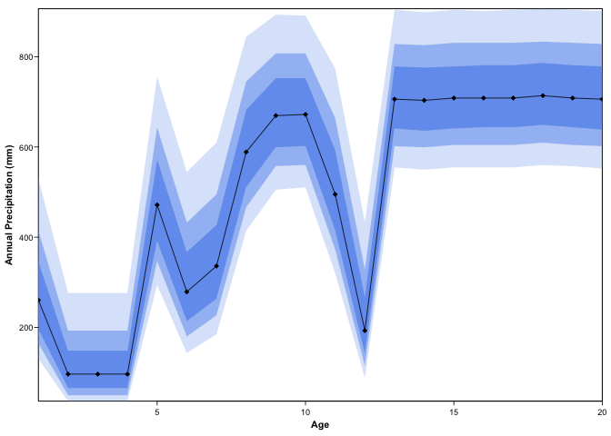
plot(recons, climate = 'bio12', simplify=TRUE, uncertainties=c(0.4, 0.6, 0.8))

If satisfying, the results can be directly exported from the R environment in unique spreadsheets for each variables (or csv files) and the crest object is exported as an RData file to enable easy reuse in the future.
export(recons, loc=getwd(), dataname='crest-test')
list.files(file.path(getwd(), 'crest-test'))
#> [1] "bio1"             "bio12"            "crest-test.RData"