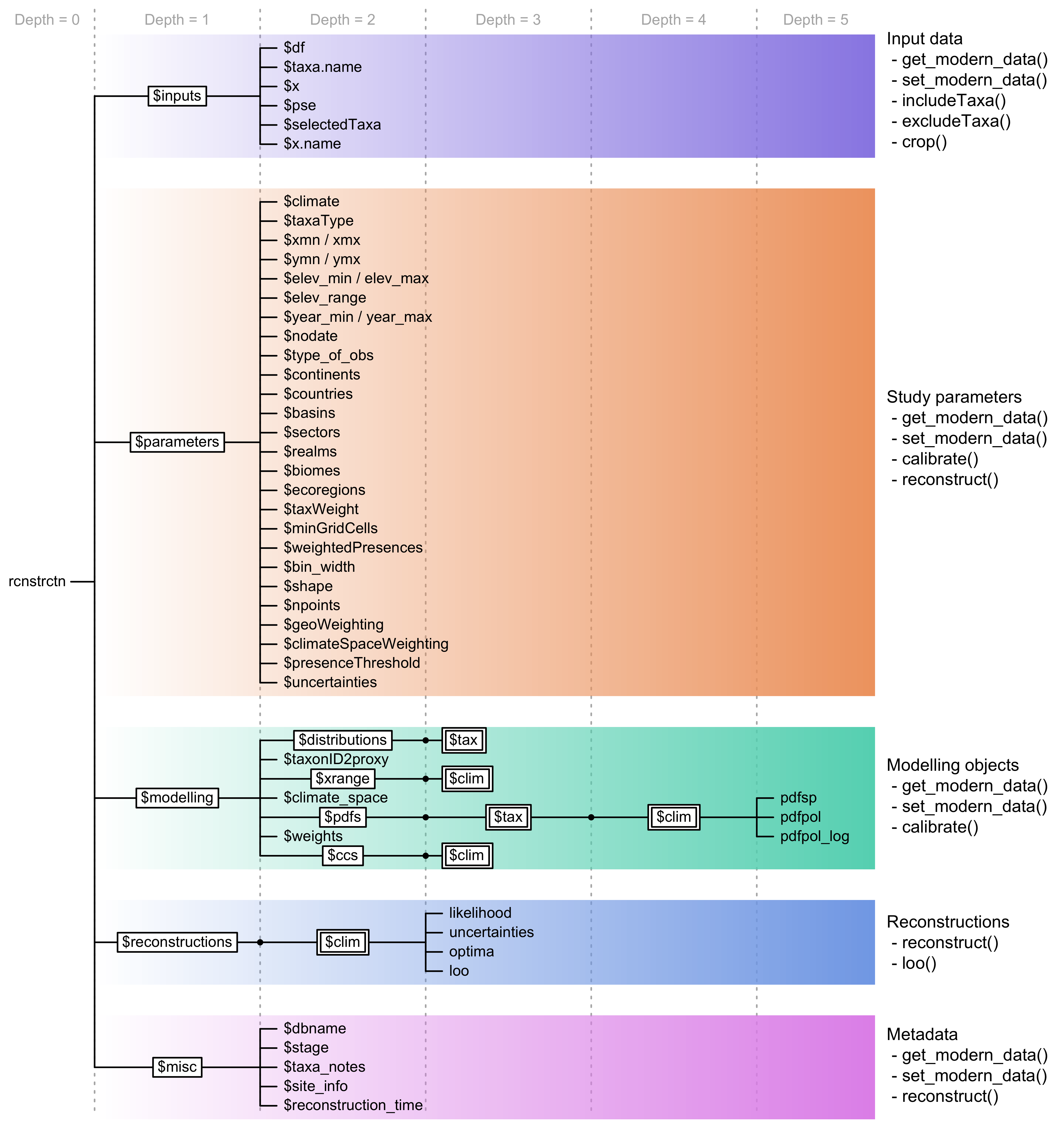
The fossil data (df)
The df data frame is only required if
crestr is used for reconstucting climate and can be omitted
if the objective is to model the climate response(s) of different taxa.
df should be a data frame with the different samples
entered as rows, with either the age, depth or sample ID as first column
and the fossil data in the subsequent columns. df can
countain raw counts, percentages, presence/absence (1s and 0s) or even
relative weights to be used in the reconstruction.
The df data frame is required if crestr is used
for reconstructing climate and can be omitted if the objective is
limited to modelling the climate response(s) of different taxa.
df is a data frame with the samples entered as rows, with
either the age, depth, or sample ID as the first column and the fossil
data in the subsequent columns. df can contain raw counts,
percentages, presence/absence (1s and 0s) or even relative weights to be
used in the reconstruction. In the case study presented here,
215 terrestrial and aquatic pollen taxa were observed in 181 samples, so
that df is a data frame with 216 columns (the age of the
samples followed by the pollen taxa) and 181 rows containing pollen
percentages of terrestrial taxa.
The proxy-species equivalency (PSE) table
The PSE data frame is required to use the
gbif4crest calibration dataset. It is used to associate
individual species available in the TAXA table with their
corresponding fossil taxon. When all the fossil taxa are identified at
the species level, the PSE table is a simple data frame
with one row per taxon (see for instance the row corresponding to
Elais guineensis in Table 1). However, fossil
taxa are most often identified at a lower taxonomic resolution
(sub-genus, genus, sub-family, family). These varying levels of
identification should be encoded in the PSE file to link
one or more (groups of) species to their common fossil taxon name
(i.e. group together all the species that are likely to have
produced the observed fossil). Several species can be assigned to a
taxon at once by limiting the taxonomic description at the family or
genus level (e.g. Artemisia in Table
1). A PSE file is composed of five columns
(Table 1). The first one (Level) contains an
integer that indicates the level of taxonomic resolution of the row (1
for Family, 2 for Genus, 3 for Species and 4 for taxa that should be
excluded from the reconstruction, e.g. ‘Triletes spores’ in the
example case study). The fifth column ProxyName contains the
name of the taxon. All the taxa recorded in the df dataset
should be listed here, or they will be excluded. Columns two to four
contain the taxonomic classification of that taxon as Family,
Genus and Species, respectively. For simplicity, a
pre-formatted version of the PSE table with the names of
all the taxa to study can be generated by crestr using the createPSE(list_of_taxa)
function that generates a spreadsheet with the correct structure and
with the Level and ProxyName columns automatically.
Table 1 Example classification of four pollen taxa
from the example case study, each one with a different level of
taxonomic resolution. The last column ‘Taxonomic resolution’ is added
here for illustrative purposes and should not included in the
PSE table.
| 1 |
Asteraceae |
|
|
Asteraceae undiff. |
Family |
| 2 |
Asteraceae |
Stoebe |
|
Stoebe-type |
Subfamily |
| 2 |
Asteraceae |
Elytropappus |
|
Stoebe-type |
Subfamily |
| 2 |
Asteraceae |
Artemisia |
|
Artemisia |
Genus level |
| 3 |
Arecaceae |
Elaeis |
Elaeis guineensis |
Elaeis guineensis |
Species |
| 4 |
|
|
|
Triletes spores |
To be excluded |
The species - taxon associated is performed in sequential steps by
the crest.get_modern_data()
function. First, crestr classifies the taxa with the lowest
taxonomical resolution (i.e. when Level is equal to
one) and then increases the resolution Level by Level.
In the example in Table 1, different taxonomic
resolution levels are provided for different plant species belonging to
the highly diverse Asteraceae family (the daisy family). To distribute
all the Asteraceae species observed across the study area to their
appropriate taxon, all the species are first classified as ‘Asteraceae
undiff.’ (first row, Level = 1). In a second time, the
classification of some of these Asteraceae species is refined when
reaching the better-resolved sub-groups (Stoebe-type and
Artemisia at Level = 2). At the end of the process,
the ‘Asteraceae undiff.’ group only contains Asteraceae species that
grow in the study area but are not part of the genera Stoebe,
Elytropappus or Artemisia. The latter are categorised
separately as Stoebe-type or Artemisia.
Additional taxa can also be added to the PSE file to
exclude species known not to be part of a group. For instance, this
‘trick’ could have been used to simplify the climate response of the
‘Asteraceae undiff.’ group by excluding more species from it, even if
the pollen grains corresponding to these species have not been observed.
This categorisation process can be time-consuming, as all the taxa must
be classified in a unique PSE table, and this process will
often require many iterations to be optimised. The results of the
different assignments are stored in the crestObj returned
by the crest.get_modern_data()
function and can be evaluated by checking
rcnstrctn$misc$taxa_notes.
