
The goal of ggcoverage is simplify the process of
visualizing genome coverage. It contains three main parts:
ggcoverage can load
BAM, BigWig (.bw), BedGraph files from various NGS data, including WGS,
RNA-seq, ChIP-seq, ATAC-seq, et al.ggcoverage supports
six different annotations:
ggcoverage utilizes ggplot2 plotting
system, so its usage is ggplot2-style!
ggcoverage is an R package distributed as part of the CRAN. To install the package,
start R and enter:
# install via CRAN
install.package("ggcoverage")

# install via Github
# install.package("remotes")   #In case you have not installed it.
remotes::install_github("showteeth/ggcoverage")
In general, it is recommended to install from Github repository (update more timely).
Once ggcoverage is installed, it can be loaded by the
following command.
library("rtracklayer")
library("ggcoverage")The RNA-seq data used here are from Transcription profiling by high throughput sequencing of HNRNPC knockdown and control HeLa cells, we select four sample to use as example: ERR127307_chr14, ERR127306_chr14, ERR127303_chr14, ERR127302_chr14, and all bam files are converted to bigwig file with deeptools.
Load metadata:
# load metadata
meta.file <- system.file("extdata", "RNA-seq", "meta_info.csv", package = "ggcoverage")
sample.meta = read.csv(meta.file)
sample.meta
#>        SampleName    Type Group
#> 1 ERR127302_chr14 KO_rep1    KO
#> 2 ERR127303_chr14 KO_rep2    KO
#> 3 ERR127306_chr14 WT_rep1    WT
#> 4 ERR127307_chr14 WT_rep2    WT
Load track files:
# track folder
track.folder = system.file("extdata", "RNA-seq", package = "ggcoverage")
# load bigwig file
track.df = LoadTrackFile(track.folder = track.folder, format = "bw",
                         meta.info = sample.meta)
# check data
head(track.df)
#>   seqnames    start      end score    Type Group
#> 1    chr14 21572751 21630650     0 KO_rep1    KO
#> 2    chr14 21630651 21630700     1 KO_rep1    KO
#> 3    chr14 21630701 21630800     4 KO_rep1    KO
#> 4    chr14 21630801 21657350     0 KO_rep1    KO
#> 5    chr14 21657351 21657450     1 KO_rep1    KO
#> 6    chr14 21657451 21663550     0 KO_rep1    KO
Prepare mark region:
# create mark region
mark.region=data.frame(start=c(21678900,21732001,21737590),
                       end=c(21679900,21732400,21737650),
                       label=c("M1", "M2", "M3"))
# check data
mark.region
#>      start      end label
#> 1 21678900 21679900    M1
#> 2 21732001 21732400    M2
#> 3 21737590 21737650    M3
Load GTF file:
gtf.file = system.file("extdata", "used_hg19.gtf", package = "ggcoverage")
gtf.gr = rtracklayer::import.gff(con = gtf.file, format = 'gtf')basic.coverage = ggcoverage(data = track.df, color = "auto",
mark.region = mark.region, range.position = "out")
basic.coverage
You can also change Y axis style:
basic.coverage = ggcoverage(data = track.df, color = "auto",
                            mark.region = mark.region, range.position = "in")
basic.coverage
basic.coverage +
  geom_gene(gtf.gr=gtf.gr)
basic.coverage +
  geom_transcript(gtf.gr=gtf.gr,label.vjust = 1.5)
basic.coverage +
  geom_gene(gtf.gr=gtf.gr) +
  geom_ideogram(genome = "hg19",plot.space = 0)
#> Loading ideogram...
#> Loading ranges...
#> Scale for 'x' is already present. Adding another scale for 'x', which will
#> replace the existing scale.
basic.coverage +
  geom_transcript(gtf.gr=gtf.gr,label.vjust = 1.5) +
  geom_ideogram(genome = "hg19",plot.space = 0)
#> Loading ideogram...
#> Loading ranges...
#> Scale for 'x' is already present. Adding another scale for 'x', which will
#> replace the existing scale.
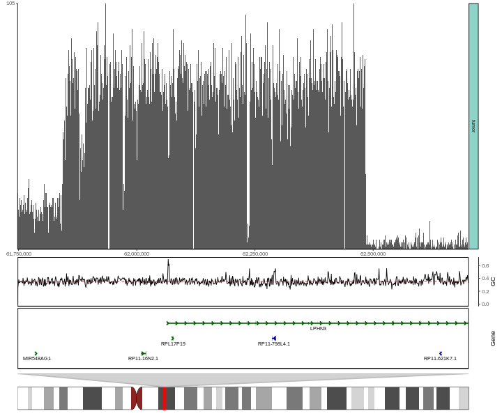
The DNA-seq data used here are from Copy
number work flow, we select tumor sample, and get bin counts with
cn.mops::getReadCountsFromBAM with WL
1000.
# track file
track.file = system.file("extdata", "DNA-seq", "CNV_example.txt", package = "ggcoverage")
track.df = read.table(track.file, header = TRUE)
# check data
head(track.df)
#>   seqnames    start      end score  Type Group
#> 1     chr4 61743001 61744000    17 tumor tumor
#> 2     chr4 61744001 61745000    14 tumor tumor
#> 3     chr4 61745001 61746000    13 tumor tumor
#> 4     chr4 61746001 61747000    16 tumor tumor
#> 5     chr4 61747001 61748000    25 tumor tumor
#> 6 chr4 61748001 61749000 24 tumor tumorbasic.coverage = ggcoverage(data = track.df,color = NULL, mark.region = NULL,
region = 'chr4:61750000-62,700,000', range.position = "out")
basic.coverage
Add GC, ideogram and gene annotaions.
# load genome data
library("BSgenome.Hsapiens.UCSC.hg19")
#> Loading required package: BSgenome
#> Loading required package: Biostrings
#> Loading required package: XVector
#>
#> Attaching package: 'Biostrings'
#> The following object is masked from 'package:base':
#>
#>     strsplit
# create plot
basic.coverage +
  geom_gc(bs.fa.seq=BSgenome.Hsapiens.UCSC.hg19) +
  geom_gene(gtf.gr=gtf.gr) +
  geom_ideogram(genome = "hg19")
#> Loading ideogram...
#> Loading ranges...
#> Scale for 'x' is already present. Adding another scale for 'x', which will
#> replace the existing scale.
# prepare sample metadata
sample.meta <- data.frame(
  SampleName = c("tumorA.chr4.selected"),
  Type = c("tumorA"),
  Group = c("tumorA")
)
# load bam file
bam.file = system.file("extdata", "DNA-seq", "tumorA.chr4.selected.bam", package = "ggcoverage")
track.df <- LoadTrackFile(
  track.file = bam.file,
  meta.info = sample.meta,
  single.nuc=TRUE, single.nuc.region="chr4:62474235-62474295"
)
head(track.df)
#>   seqnames    start      end score   Type  Group
#> 1     chr4 62474235 62474236     5 tumorA tumorA
#> 2     chr4 62474236 62474237     5 tumorA tumorA
#> 3     chr4 62474237 62474238     5 tumorA tumorA
#> 4     chr4 62474238 62474239     6 tumorA tumorA
#> 5     chr4 62474239 62474240     6 tumorA tumorA
#> 6 chr4 62474240 62474241 6 tumorA tumorAFor base and amino acid annotation, we have following default color
schemes, you can change with nuc.color and
aa.color parameters.
Default color scheme for base annotation is
Clustal-style, more popular color schemes is available here.
# color scheme
nuc.color = c("A" = "#ff2b08", "C" = "#009aff", "G" = "#ffb507", "T" = "#00bc0d")
# create plot
graphics::par(mar = c(1, 5, 1, 1))
graphics::image(
  1:length(nuc.color), 1, as.matrix(1:length(nuc.color)),
  col = nuc.color,
  xlab = "", ylab = "", xaxt = "n", yaxt = "n", bty = "n"
)
graphics::text(1:length(nuc.color), 1, names(nuc.color))
graphics::mtext(
  text = "Base", adj = 1, las = 1,
  side = 2
)
Default color scheme for amino acid annotation is from Residual colours: a proposal for aminochromography:
aa.color = c(
  "D" = "#FF0000", "S" = "#FF2400", "T" = "#E34234", "G" = "#FF8000", "P" = "#F28500",
  "C" = "#FFFF00", "A" = "#FDFF00", "V" = "#E3FF00", "I" = "#C0FF00", "L" = "#89318C",
  "M" = "#00FF00", "F" = "#50C878", "Y" = "#30D5C8", "W" = "#00FFFF", "H" = "#0F2CB3",
  "R" = "#0000FF", "K" = "#4b0082", "N" = "#800080", "Q" = "#FF00FF", "E" = "#8F00FF",
  "*" = "#FFC0CB", " " = "#FFFFFF", " " = "#FFFFFF", " " = "#FFFFFF", " " = "#FFFFFF"
)

graphics::par(mar = c(1, 5, 1, 1))
graphics::image(
  1:5, 1:5, matrix(1:length(aa.color),nrow=5),
  col = rev(aa.color),
  xlab = "", ylab = "", xaxt = "n", yaxt = "n", bty = "n"
)
graphics::text(expand.grid(1:5,1:5), names(rev(aa.color)))
graphics::mtext(
  text = "Amino acids", adj = 1, las = 1,
  side = 2
)
ggcoverage(data = track.df, color = "grey", range.position = "out", single.nuc=T, rect.color = "white") +
  geom_base(bam.file = bam.file,
            bs.fa.seq = BSgenome.Hsapiens.UCSC.hg19) +
  geom_ideogram(genome = "hg19",plot.space = 0)
#> Loading ideogram...
#> Loading ranges...
#> Scale for 'x' is already present. Adding another scale for 'x', which will
#> replace the existing scale.
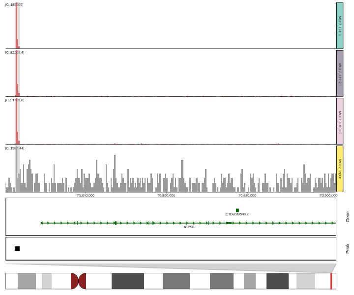
The ChIP-seq data used here are from DiffBind, I select four sample to use as example: Chr18_MCF7_input, Chr18_MCF7_ER_1, Chr18_MCF7_ER_3, Chr18_MCF7_ER_2, and all bam files are converted to bigwig file with deeptools.
Create metadata:
# load metadata
sample.meta = data.frame(SampleName=c('Chr18_MCF7_ER_1','Chr18_MCF7_ER_2','Chr18_MCF7_ER_3','Chr18_MCF7_input'),
                         Type = c("MCF7_ER_1","MCF7_ER_2","MCF7_ER_3","MCF7_input"),
                         Group = c("IP", "IP", "IP", "Input"))
sample.meta
#>         SampleName       Type Group
#> 1  Chr18_MCF7_ER_1  MCF7_ER_1    IP
#> 2  Chr18_MCF7_ER_2  MCF7_ER_2    IP
#> 3  Chr18_MCF7_ER_3  MCF7_ER_3    IP
#> 4 Chr18_MCF7_input MCF7_input Input
Load track files:
# track folder
track.folder = system.file("extdata", "ChIP-seq", package = "ggcoverage")
# load bigwig file
track.df = LoadTrackFile(track.folder = track.folder, format = "bw",
                         meta.info = sample.meta)
# check data
head(track.df)
#>   seqnames    start      end   score      Type Group
#> 1    chr18 76799701 76800000 439.316 MCF7_ER_1    IP
#> 2    chr18 76800001 76800300 658.974 MCF7_ER_1    IP
#> 3    chr18 76800301 76800600 219.658 MCF7_ER_1    IP
#> 4    chr18 76800601 76800900 658.974 MCF7_ER_1    IP
#> 5    chr18 76800901 76801200   0.000 MCF7_ER_1    IP
#> 6    chr18 76801201 76801500 219.658 MCF7_ER_1    IP
Prepare mark region:
# create mark region
mark.region=data.frame(start=c(76822533),
                       end=c(76823743),
                       label=c("Promoter"))
# check data
mark.region
#>      start      end    label
#> 1 76822533 76823743 Promoterbasic.coverage = ggcoverage(data = track.df, color = "auto", region = "chr18:76822285-76900000",
mark.region=mark.region, show.mark.label = FALSE)
basic.coverage
Add gene, ideogram and peak annotations. To create peak annotation, we first get consensus peaks with MSPC.
# get consensus peak file
peak.file = system.file("extdata", "ChIP-seq", "consensus.peak", package = "ggcoverage")

basic.coverage +
  geom_gene(gtf.gr=gtf.gr) +
  geom_peak(bed.file = peak.file) +
  geom_ideogram(genome = "hg19",plot.space = 0)
#> Loading ideogram...
#> Loading ranges...
#> Scale for 'x' is already present. Adding another scale for 'x', which will
#> replace the existing scale.
Please note that the ggcoverage project is released with
a Contributor
Code of Conduct. By contributing to this project, you agree to abide
by its terms.