![]()
![]()
ggtikz allows you to annotate plots created using ggplot2 with arbitrary TikZ code when rendering them with the tikzDevice. The annotations can be made using data coordinates, or with coordinates relative to a specified panel or the whole plot.
Plots with multiple panels (via facet_grid() or
facet_wrap()) are supported.
For a few examples, see the examples vignette.
You can install the latest ggtikz release from CRAN with:
install.packages("ggtikz")Or get the development version from GitHub:
# install.packages("devtools")
devtools::install_github("osthomas/ggtikz", ref = "devel")ggtikz().library(ggplot2)
library(ggtikz)
p <- ggplot(mtcars, aes(disp, mpg)) + geom_point() # 1.
## tikz("plot.tikz")
ggtikz(p,
"\\fill[red] (0.5,0.5) circle (5mm);",
xy = "panel", panelx = 1, panely = 1)
## dev.off()
## Render with LaTeX ...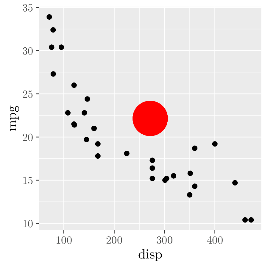
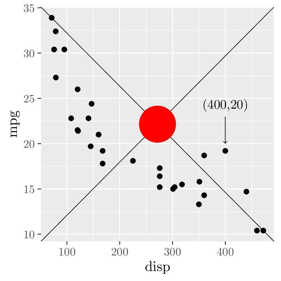
ggtikzCanvas().ggtikzAnnotation().library(ggplot2)
library(ggtikz)
p <- ggplot(mtcars, aes(disp, mpg)) + geom_point() # 1.
canvas <- ggtikzCanvas(p) # 2.
annot1 <- ggtikzAnnotation( # 3.
"
\\draw (0,0) -- (1,1);
\\draw (0,1) -- (1,0);
\\fill[red] (0.5,0.5) circle (5mm);
",
xy = "panel", panelx = 1, panely = 1
)
annot2 <- ggtikzAnnotation( # 3.
"\\draw[<-] (400,20) -- ++(0,3) node[at end, anchor=south] {(400,20)};",
xy = "data", panelx = 1, panely = 1
)
## tikz("plot.tikz")
p # 4. + 5.
canvas + annot1 + annot2
## dev.off()
## Render with LaTeX ...