marginaleffects package for R

marginaleffects package for R
![]()
![]()
Compute and plot adjusted predictions, contrasts, marginal effects,
and marginal means for 68classes of statistical models in
R. Conduct linear and non-linear hypothesis tests using the
delta method.
Introduction:
Vignettes:
Case studies:
brmsTips and technical notes:
External links:
The marginaleffects package allows R users
to compute and plot four principal quantities of interest for 68
different classes of models:
predictions(),
plot_cap()marginaleffects(),
plot(),
plot_cme()comparisons(),
plot_cco()marginalmeans()One confusing aspect of the definitions above is that they use the word “marginal” in two different and opposite ways:
Another potential confusion arises when some analysts use “marginal” to distinguish some estimates from “conditional” ones. As noted in the marginal effects and the contrasts vignettes, slopes and contrasts often vary from individual to individual, based on the values of all the regressors in the model. When we estimate a slope or a contrast for a specific combination of predictors – for one (possibly representative) individual – some people will call this a “conditional” estimate. When we compute the average of several individual-level estimates, some people will call this a “marginal” estimate.
On this website and in this package, we will reserve the expression “marginal effect” to mean a “slope” or “derivative”. When we take the average unit-level estimates, we will call this an “average marginal effect.”
This is all very confusing, but the terminology is so widespread and inconsistent that we must press on…
To calculate marginal effects we need to take derivatives of the regression equation. This can be challenging to do manually, especially when our models are non-linear, or when regressors are transformed or interacted. Computing the variance of a marginal effect is even more difficult.
The marginaleffects package hopes to do most of this
hard work for you.
Many R packages advertise their ability to compute
“marginal effects.” However, most of them do not actually
compute marginal effects as defined above. Instead, they
compute “adjusted predictions” for different regressor values, or
differences in adjusted predictions (i.e., “contrasts”). The rare
packages that actually compute marginal effects are typically limited in
the model types they support, and in the range of transformations they
allow (interactions, polynomials, etc.).
The main packages in the R ecosystem to compute marginal
effects are the trailblazing and powerful margins
by Thomas J. Leeper, and emmeans
by Russell V. Lenth and contributors. The
marginaleffects package is essentially a clone of
margins, with some additional features from
emmeans.
So why did I write a clone?
Stata, or other R
packages.ggplot2 support for plotting
(conditional) marginal effects and adjusted predictions.marginaleffects
follow “tidy” principles. They are easy to program with and feed to other
packages like modelsummary.Downsides of marginaleffects include:
You can install the released version of marginaleffects
from CRAN:
install.packages("marginaleffects")You can install the development version of
marginaleffects from Github:
remotes::install_github("vincentarelbundock/marginaleffects")First, we estimate a linear regression model with multiplicative interactions:
library(marginaleffects)

mod <- lm(mpg ~ hp * wt * am, data = mtcars)An “adjusted prediction” is the outcome predicted by a model for some combination of the regressors’ values, such as their observed values, their means, or factor levels (a.k.a. “reference grid”).
By default, the predictions() function returns adjusted
predictions for every value in original dataset:
predictions(mod) |> head()
#>   rowid     type predicted std.error statistic       p.value conf.low conf.high
#> 1     1 response  22.48857 0.8841487  25.43528 1.027254e-142 20.66378  24.31336
#> 2     2 response  20.80186 1.1942050  17.41900  5.920119e-68 18.33714  23.26658
#> 3     3 response  25.26465 0.7085307  35.65781 1.783452e-278 23.80232  26.72699
#> 4     4 response  20.25549 0.7044641  28.75305 8.296026e-182 18.80155  21.70943
#> 5     5 response  16.99782 0.7118658  23.87784 5.205109e-126 15.52860  18.46704
#> 6     6 response  19.66353 0.8753226  22.46433 9.270636e-112 17.85696  21.47011
#>    mpg  hp    wt am
#> 1 21.0 110 2.620  1
#> 2 21.0 110 2.875  1
#> 3 22.8  93 2.320  1
#> 4 21.4 110 3.215  0
#> 5 18.7 175 3.440  0
#> 6 18.1 105 3.460  0
The datagrid
function gives us a powerful way to define a grid of predictors. All
the variables not mentioned explicitly in datagrid() are
fixed to their mean or mode:
predictions(mod, newdata = datagrid(am = 0, wt = seq(2, 3, .2)))
#>   rowid     type predicted std.error statistic       p.value conf.low conf.high
#> 1     1 response  21.95621 2.0386301  10.77008  4.765935e-27 17.74868  26.16373
#> 2     2 response  21.42097 1.7699036  12.10290  1.019401e-33 17.76807  25.07388
#> 3     3 response  20.88574 1.5067373  13.86157  1.082834e-43 17.77599  23.99549
#> 4     4 response  20.35051 1.2526403  16.24609  2.380723e-59 17.76518  22.93583
#> 5     5 response  19.81527 1.0144509  19.53301  5.755097e-85 17.72155  21.90900
#> 6     6 response  19.28004 0.8063905  23.90906 2.465206e-126 17.61573  20.94435
#>         hp am  wt
#> 1 146.6875  0 2.0
#> 2 146.6875  0 2.2
#> 3 146.6875  0 2.4
#> 4 146.6875  0 2.6
#> 5 146.6875  0 2.8
#> 6 146.6875  0 3.0
We can plot how predictions change for different values of one or
more variables – Conditional Adjusted Predictions – using the
plot_cap function:
plot_cap(mod, condition = c("hp", "wt"))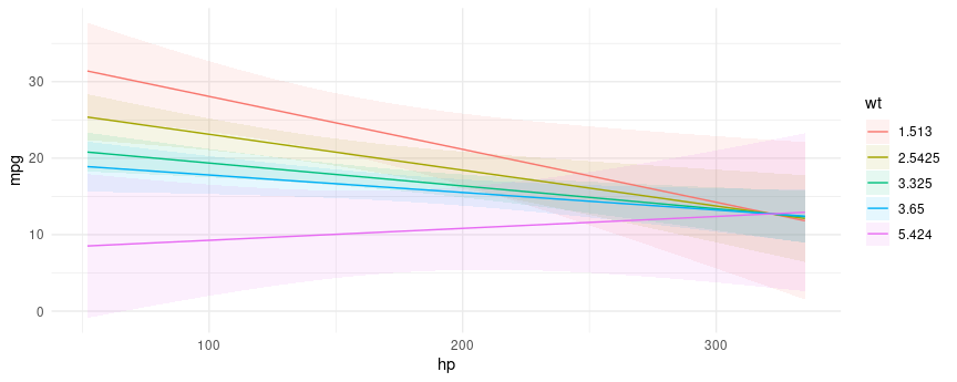
mod2 <- lm(mpg ~ factor(cyl), data = mtcars)
plot_cap(mod2, condition = "cyl")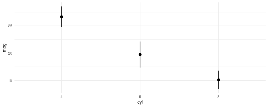
The
Adjusted Predictions vignette shows how to use the
predictions() and plot_cap() functions to
compute a wide variety of quantities of interest:
A contrast is the difference between two adjusted predictions, calculated for meaningfully different predictor values (e.g., College graduates vs. Others).
What happens to the predicted outcome when a numeric predictor increases by one unit, and logical variable flips from FALSE to TRUE, and a factor variable shifts from baseline?
titanic <- read.csv("https://vincentarelbundock.github.io/Rdatasets/csv/Stat2Data/Titanic.csv")
titanic$Woman <- titanic$Sex == "female"
mod3 <- glm(Survived ~ Woman + Age * PClass, data = titanic, family = binomial)

cmp <- comparisons(mod3)
summary(cmp)
#>     Term     Contrast   Effect Std. Error z value   Pr(>|z|)     2.5 %
#> 1  Woman TRUE - FALSE  0.50329   0.031654  15.899 < 2.22e-16  0.441244
#> 2    Age  (x + 1) - x -0.00558   0.001084  -5.147 2.6471e-07 -0.007705
#> 3 PClass    2nd - 1st -0.22603   0.043546  -5.191 2.0950e-07 -0.311383
#> 4 PClass    3rd - 1st -0.38397   0.041845  -9.176 < 2.22e-16 -0.465985
#>      97.5 %
#> 1  0.565327
#> 2 -0.003455
#> 3 -0.140686
#> 4 -0.301957
#>
#> Model type:  glm
#> Prediction type:  response
The contrast above used a simple difference between adjusted
predictions. We can also used different functions to combine and
contrast predictions in different ways. For instance, researchers often
compute Adjusted Risk Ratios, which are ratios of predicted
probabilities. We can compute such ratios by applying a transformation
using the transform_pre argument. We can also present the
results of “interactions” between contrasts. What happens to the ratio
of predicted probabilities for survival when PClass changes
between each pair of factor levels (“pairwise”) and Age
changes by 2 standard deviations simultaneously:
cmp <- comparisons(
    mod3,
    transform_pre = "ratio",
    variables = list(Age = "2sd", PClass = "pairwise"))
summary(cmp)
#>                   Age    PClass Effect Std. Error z value   Pr(>|z|)  2.5 %
#> 1 (x - sd) / (x + sd) 1st / 1st 0.7043    0.05946  11.846 < 2.22e-16 0.5878
#> 2 (x - sd) / (x + sd) 2nd / 1st 0.3185    0.05566   5.723 1.0442e-08 0.2095
#> 3 (x - sd) / (x + sd) 3rd / 1st 0.2604    0.05308   4.907 9.2681e-07 0.1564
#> 4 (x - sd) / (x + sd) 2nd / 2nd 0.3926    0.08101   4.846 1.2588e-06 0.2338
#> 5 (x - sd) / (x + sd) 3rd / 2nd 0.3162    0.07023   4.503 6.7096e-06 0.1786
#> 6 (x - sd) / (x + sd) 3rd / 3rd 0.7053    0.20273   3.479 0.00050342 0.3079
#>   97.5 %
#> 1 0.8209
#> 2 0.4276
#> 3 0.3645
#> 4 0.5514
#> 5 0.4539
#> 6 1.1026
#>
#> Model type:  glm
#> Prediction type:  response
The code above is explained in detail in the vignette on Transformations and Custom Contrasts.
The
Contrasts vignette shows how to use the comparisons()
function to compute a wide variety of quantities of interest:
A “marginal effect” is a partial derivative (slope) of the regression
equation with respect to a regressor of interest. It is unit-specific
measure of association between a change in a regressor and a change in
the regressand. The marginaleffects() function uses
numerical derivatives to estimate the slope of the regression equation
with respect to each of the variables in the model (or contrasts for
categorical variables).
By default, marginaleffects() estimates the slope for
each row of the original dataset that was used to fit the model:
mfx <- marginaleffects(mod)

head(mfx, 4)
#>   rowid     type term        dydx  std.error statistic     p.value    conf.low
#> 1     1 response   hp -0.03690556 0.01850172 -1.994710 0.046074551 -0.07316825
#> 2     2 response   hp -0.02868936 0.01562861 -1.835695 0.066402771 -0.05932087
#> 3     3 response   hp -0.04657166 0.02258715 -2.061866 0.039220507 -0.09084166
#> 4     4 response   hp -0.04227128 0.01328278 -3.182412 0.001460541 -0.06830506
#>       conf.high predicted_lo predicted_hi  mpg  hp    wt am    eps
#> 1 -0.0006428553     22.48857     22.48752 21.0 110 2.620  1 0.0283
#> 2  0.0019421508     20.80186     20.80105 21.0 110 2.875  1 0.0283
#> 3 -0.0023016728     25.26465     25.26333 22.8  93 2.320  1 0.0283
#> 4 -0.0162375066     20.25549     20.25430 21.4 110 3.215  0 0.0283
The function summary calculates the “Average Marginal
Effect,” that is, the average of all unit-specific marginal effects:
summary(mfx)
#>   Term   Effect Std. Error  z value   Pr(>|z|)    2.5 %   97.5 %
#> 1   hp -0.03807    0.01279 -2.97725 0.00290848 -0.06314 -0.01301
#> 2   wt -3.93909    1.08596 -3.62728 0.00028642 -6.06754 -1.81065
#> 3   am -0.04811    1.85260 -0.02597 0.97928234 -3.67913  3.58292
#>
#> Model type:  lm
#> Prediction type:  response
The plot_cme plots “Conditional Marginal Effects,” that
is, the marginal effects estimated at different values of a regressor
(often an interaction):
plot_cme(mod, effect = "hp", condition = c("wt", "am"))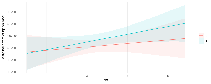
The
Marginal Effects vignette shows how to use the
marginaleffects() function to compute a wide variety of
quantities of interest:
Marginal Means are the adjusted predictions of a model, averaged across a “reference grid” of categorical predictors. To compute marginal means, we first need to make sure that the categorical variables of our model are coded as such in the dataset:
dat <- mtcars
dat$am <- as.logical(dat$am)
dat$cyl <- as.factor(dat$cyl)
Then, we estimate the model and call the marginalmeans
function:
mod <- lm(mpg ~ am + cyl + hp, data = dat)
mm <- marginalmeans(mod)
summary(mm)
#>   Term Value  Mean Std. Error z value   Pr(>|z|) 2.5 % 97.5 %
#> 1   am FALSE 18.32     0.7854   23.33 < 2.22e-16 16.78  19.86
#> 2   am  TRUE 22.48     0.8343   26.94 < 2.22e-16 20.84  24.11
#> 3  cyl     4 22.88     1.3566   16.87 < 2.22e-16 20.23  25.54
#> 4  cyl     6 18.96     1.0729   17.67 < 2.22e-16 16.86  21.06
#> 5  cyl     8 19.35     1.3771   14.05 < 2.22e-16 16.65  22.05
#>
#> Model type:  lm
#> Prediction type:  response
#> Results averaged over levels of: am, cyl
The Marginal Means vignette offers more detail.
There is much more you can do with
marginaleffects. Return to the Table
of Contents to read the vignettes, learn how to report marginal
effects and means in nice tables
with the modelsummary package, how to define your own
prediction “grid”, and much more.