The goal of pivmet is to propose some pivotal methods in order to:
undo the label switching problem which naturally arises during the MCMC sampling in Bayesian mixture models () pivotal relabelling (Egidi et al. 2018a)
initialize the K-means algorithm aimed at obtaining a good clustering solution () pivotal seeding (Egidi et al. 2018b)
You can then install pivmet from github with:
First of all, we load the package and we import the fish dataset belonging to the bayesmix package:
library(pivmet)
#> Loading required package: bayesmix
#> Loading required package: rjags
#> Loading required package: coda
#> Linked to JAGS 4.3.0
#> Loaded modules: basemod,bugs
#> Loading required package: mvtnorm
#> Loading required package: RcmdrMisc
#> Loading required package: car
#> Loading required package: carData
#> Loading required package: sandwich
#> Warning: replacing previous import 'rstan::plot' by 'graphics::plot' when
#> loading 'pivmet'
data(fish)
y <- fish[,1]
N <- length(y)  # sample size
k <- 5          # fixed number of clusters
nMC <- 12000    # MCMC iterations
Then we fit a Bayesian Gaussian mixture using the piv_MCMC function:
res <- piv_MCMC(y = y, k = k, nMC = nMC)
#> Compiling model graph
#>    Declaring variables
#>    Resolving undeclared variables
#>    Allocating nodes
#> Graph information:
#>    Observed stochastic nodes: 256
#>    Unobserved stochastic nodes: 268
#>    Total graph size: 1050
#>
#> Initializing model
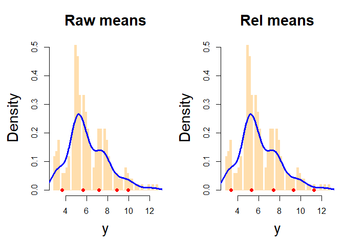
Finally, we can apply pivotal relabelling and inspect the new posterior estimates with the functions piv_rel and piv_plot, respectively:

#> Description: traceplots of the raw MCMC chains and the relabelled chains for all the model parameters: means, sds and weights. Each colored chain corresponds to one of the k distinct parameters of the mixture model. Overlapping chains may reveal that the MCMC sampler is not able to distinguish between the components.
piv_plot(y = y, mcmc = res, rel_est = rel, type = "hist")
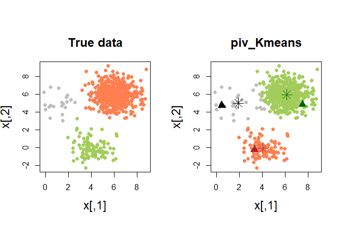
#> Description: histograms of the data along with the estimated posterior means (red points) from raw MCMC and relabelling algorithm. The blue line is the estimated density curve.Sometimes K-means algorithm does not provide an optimal clustering solution. Suppose to generate some clustered data and to detect one pivotal unit for each group with the MUS (Maxima Units Search algorithm) function:
#generate some data

set.seed(123)
n  <- 620
centers  <- 3
n1 <- 20
n2 <- 100
n3 <- 500
x  <- matrix(NA, n,2)
truegroup <- c( rep(1,n1), rep(2, n2), rep(3, n3))

for (i in 1:n1){
 x[i,]=rmvnorm(1, c(1,5), sigma=diag(2))}
for (i in 1:n2){
 x[n1+i,]=rmvnorm(1, c(4,0), sigma=diag(2))}
for (i in 1:n3){
 x[n1+n2+i,]=rmvnorm(1, c(6,6), sigma=diag(2))}

H <- 1000
a <- matrix(NA, H, n)

  for (h in 1:H){
    a[h,] <- kmeans(x,centers)$cluster
  }

#build the similarity matrix
sim_matr <- matrix(1, n,n)
 for (i in 1:(n-1)){
    for (j in (i+1):n){
      sim_matr[i,j] <- sum(a[,i]==a[,j])/H
      sim_matr[j,i] <- sim_matr[i,j]
    }
  }

cl <- KMeans(x, centers)$cluster
mus_alg <- MUS(C = sim_matr, clusters = cl, prec_par = 5)
Quite often, classical K-means fails in recognizing the true groups:
# launch classical KMeans
kmeans_res <- KMeans(x, centers)
# plots
par(mfrow=c(1,2))
colors_cluster <- c("grey", "darkolivegreen3", "coral")
colors_centers <- c("black", "darkgreen", "firebrick")

graphics::plot(x, col = colors_cluster[truegroup]
                 ,bg= colors_cluster[truegroup], pch=21,
                  xlab="y[,1]",
                  ylab="y[,2]", cex.lab=1.5,
                  main="True data", cex.main=1.5)

graphics::plot(x, col = colors_cluster[kmeans_res$cluster],
      bg=colors_cluster[kmeans_res$cluster], pch=21, xlab="y[,1]",
      ylab="y[,2]", cex.lab=1.5,main="K-means",  cex.main=1.5)
points(kmeans_res$centers, col = colors_centers[1:centers],
      pch = 8, cex = 2)
In such situations, we may need a more robust version of the classical K-means. The pivots may be used as initial seeds for a classical K-means algorithm. The function piv_KMeans works as the classical kmeans function, with some optional arguments (in the figure below, the colored triangles represent the pivots).
# launch piv_KMeans
piv_res <- piv_KMeans(x, centers)
# plots
par(mfrow=c(1,2), pty="s")
colors_cluster <- c("grey", "darkolivegreen3", "coral")
colors_centers <- c("black", "darkgreen", "firebrick")
graphics::plot(x, col = colors_cluster[truegroup],
   bg= colors_cluster[truegroup], pch=21, xlab="x[,1]",
   ylab="x[,2]", cex.lab=1.5,
   main="True data", cex.main=1.5)

graphics::plot(x, col = colors_cluster[piv_res$cluster],
   bg=colors_cluster[piv_res$cluster], pch=21, xlab="x[,1]",
   ylab="x[,2]", cex.lab=1.5,
   main="piv_Kmeans", cex.main=1.5)
points(x[piv_res$pivots[1],1], x[piv_res$pivots[1],2],
   pch=24, col=colors_centers[1],bg=colors_centers[1],
   cex=1.5)
points(x[piv_res$pivots[2],1], x[piv_res$pivots[2],2],
   pch=24,  col=colors_centers[2], bg=colors_centers[2],
   cex=1.5)
points(x[piv_res$pivots[3],1], x[piv_res$pivots[3],2],
   pch=24, col=colors_centers[3], bg=colors_centers[3],
   cex=1.5)
points(piv_res$centers, col = colors_centers[1:centers],
   pch = 8, cex = 2)
Egidi, L., Pappadà, R., Pauli, F. and Torelli, N. (2018a). Relabelling in Bayesian Mixture Models by Pivotal Units. Statistics and Computing, 28(4), 957-969.
Egidi, L., Pappadà, R., Pauli, F., Torelli, N. (2018b). K-means seeding via MUS algorithm. Conference Paper, Book of Short Papers, SIS2018, ISBN: 9788891910233.