![]()
![]()
The goal of scrutiny is to test published summary statistics for consistency using techniques like GRIM and to check their plausibility by reconstructing some of the processes behind them. The package makes these methods easy to use in a tidyverse-friendly way. It hopes to help the new field of error detection go mainstream.
Besides ready-made tests, scrutiny features a complete system for implementing new consistency tests, more general infrastructure for implementing error detection techniques, as well as specialized data wrangling functions. See the Articles tab for vignettes.
scrutiny is a work in progress. You are welcome to contribute with pull requests. However, please open an issue first.
The package is not on CRAN yet. You can install in from GitHub like this:
remotes::install_github("lhdjung/scrutiny")Here is how to GRIM-test all values in a data frame. When using
grim_map(), the consistency column tells you
if the means (x), sample sizes (n), and
numbers of scale items are mutually consistent. Scale item numbers are 1
by default.
library(scrutiny)

# Example data:
pigs1
#> # A tibble: 12 × 2
#>    x         n
#>    <chr> <dbl>
#>  1 7.22     32
#>  2 4.74     25
#>  3 5.23     29
#>  4 2.57     24
#>  5 6.77     27
#>  6 2.68     28
#>  7 7.01     29
#>  8 7.38     26
#>  9 3.14     27
#> 10 6.89     31
#> 11 5.00     25
#> 12 0.24     28

# GRIM-testing for data frames:
grim_map(pigs1)
#> # A tibble: 12 × 4
#>    x         n consistency ratio
#>    <chr> <dbl> <lgl>       <dbl>
#>  1 7.22     32 TRUE         0.68
#>  2 4.74     25 FALSE        0.75
#>  3 5.23     29 FALSE        0.71
#>  4 2.57     24 FALSE        0.76
#>  5 6.77     27 FALSE        0.73
#>  6 2.68     28 TRUE         0.72
#>  7 7.01     29 FALSE        0.71
#>  8 7.38     26 TRUE         0.74
#>  9 3.14     27 FALSE        0.73
#> 10 6.89     31 FALSE        0.69
#> 11 5.00     25 TRUE         0.75
#> 12 0.24     28 FALSE        0.72
Test percentages instead of means:
pigs2
#> # A tibble: 6 × 2
#>   x         n
#>   <chr> <dbl>
#> 1 67.4    150
#> 2 54.2    150
#> 3 54.0    150
#> 4 69.8    150
#> 5 68.1    150
#> 6 55.4    150

grim_map(pigs2, percent = TRUE)
#> ℹ `x` converted from percentage
#> # A tibble: 6 × 4
#>   x         n consistency ratio
#>   <chr> <dbl> <lgl>       <dbl>
#> 1 0.674   150 FALSE        0.85
#> 2 0.542   150 FALSE        0.85
#> 3 0.540   150 TRUE         0.85
#> 4 0.698   150 FALSE        0.85
#> 5 0.681   150 FALSE        0.85
#> 6 0.554   150 FALSE        0.85
You can choose how the means are reconstructed for testing — here, rounded up from 5. When visualizing results, the plot will adjust automatically. Blue dots are consistent values, red dots are inconsistent ones:
pigs1 %>%
  grim_map(rounding = "up") %>%
  grim_plot()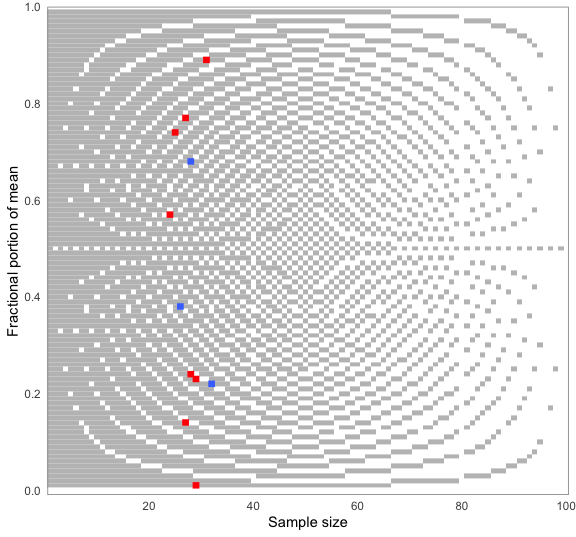
Similarly, use DEBIT to test means and standard deviations of binary data:
pigs3
#> # A tibble: 7 × 3
#> x sd n
#> <chr> <chr> <dbl>
#> 1 0.53 0.50 1683
#> 2 0.44 0.50 1683
#> 3 0.77 0.42 1683
#> 4 0.19 0.35 1683
#> 5 0.34 0.47 1683
#> 6 0.93 0.25 1683
#> 7 0.12 0.33 1683
pigs3 %>%
debit_map()
#> # A tibble: 7 × 11
#> x sd n consistency rounding sd_lo…¹ sd_in…² sd_up…³ sd_in…⁴ x_lower
#> <chr> <chr> <int> <lgl> <chr> <dbl> <lgl> <dbl> <lgl> <dbl>
#> 1 0.53 0.50 1683 TRUE up_or_d… 0.495 TRUE 0.505 TRUE 0.525
#> 2 0.44 0.50 1683 TRUE up_or_d… 0.495 TRUE 0.505 TRUE 0.435
#> 3 0.77 0.42 1683 TRUE up_or_d… 0.415 TRUE 0.425 TRUE 0.765
#> 4 0.19 0.35 1683 FALSE up_or_d… 0.345 TRUE 0.355 TRUE 0.185
#> 5 0.34 0.47 1683 TRUE up_or_d… 0.465 TRUE 0.475 TRUE 0.335
#> 6 0.93 0.25 1683 TRUE up_or_d… 0.245 TRUE 0.255 TRUE 0.925
#> 7 0.12 0.33 1683 TRUE up_or_d… 0.325 TRUE 0.335 TRUE 0.115
#> # … with 1 more variable: x_upper <dbl>, and abbreviated variable names
#> # ¹sd_lower, ²sd_incl_lower, ³sd_upper, ⁴sd_incl_upper
#> # ℹ Use `colnames()` to see all variable names
pigs3 %>%
debit_map() %>%
debit_plot()
(…) a critical inspection of the published literature should not be mischaracterized as a hobby for the overly cynical, nor as so-called “methodological terrorism”. On the contrary, carefully evaluating presented data is a cornerstone of scientific investigation, and it is only logical to apply this also to the published literature. If we are not willing to critically assess published studies, we also cannot guarantee their veracity.
— van der Zee et al. (2017, pp. 8-9)
(…) data thugs (…) demand data and if they do not receive it, they contact editors and universities and threaten to write blogs and tweets about the errors uncovered.
— Eric A. Stewart (six retractions; quoted in Pickett 2020, p. 178)
Pickett, J. T. (2020). The Stewart Retractions: A Quantitative and Qualitative Analysis. Econ Journal Watch, 17(1), 152–190. https://econjwatch.org/articles/the-stewart-retractions-a-quantitative-and-qualitative-analysis.
van der Zee, T., Anaya, J., & Brown, N. J. L. (2017). Statistical heartburn: An attempt to digest four pizza publications from the Cornell Food and Brand Lab. BMC Nutrition, 3(1), 54. https://doi.org/10.1186/s40795-017-0167-x.