Computation of sparse portfolios for financial index tracking, i.e., joint selection of a subset of the assets that compose the index and computation of their relative weights (capital allocation). The level of sparsity of the portfolios, i.e., the number of selected assets, is controlled through a regularization parameter. Different tracking measures are available, namely, the empirical tracking error (ETE), downside risk (DR), Huber empirical tracking error (HETE), and Huber downside risk (HDR). See vignette for a detailed documentation and comparison, with several illustrative examples.
The package is based on the paper:
K. Benidis, Y. Feng, and D. P. Palomar, “Sparse Portfolios for High-Dimensional Financial Index Tracking,” IEEE Trans. on Signal Processing, vol. 66, no. 1, pp. 155-170, Jan. 2018. (https://doi.org/10.1109/TSP.2017.2762286)
The latest stable version of sparseIndexTracking is available at https://CRAN.R-project.org/package=sparseIndexTracking.
The latest development version of sparseIndexTracking is available at https://github.com/dppalomar/sparseIndexTracking.
To install the latest stable version of sparseIndexTracking from CRAN, run the following commands in R:
To install the development version of sparseIndexTracking from GitHub, run the following commands in R:
To get help:
library(sparseIndexTracking)
help(package = "sparseIndexTracking")
package?sparseIndexTracking
?spIndexTrack
Please cite sparseIndexTracking in publications:
For more detailed information, please check the vignette: CRAN vignette and GitHub vignette.
spIndexTrack()We start by loading the package and real data of the index S&P 500 and its underlying assets:
The data INDEX_2010 contains a list with two xts objects:
X: A T × N xts with the daily linear returns of the N assets that were in the index during the year 2010 (total T trading days)SP500: A T × 1 xts with the daily linear returns of the index S&P 500 during the same period.
Note that we use xts objects just for illustration purposes. The function spIndexTracking() can also be invoked passing simple data arrays or dataframes.
Based on the above quantities we create a training window, which we will use to create our portfolios, and a testing window, which will be used to assess the performance of the designed portfolios. For simplicity, here we consider the first six (trading) months of the dataset (~126 days) as the training window, and the subsequent six months as the testing window:
X_train <- INDEX_2010$X[1:126]
X_test <- INDEX_2010$X[127:252]
r_train <- INDEX_2010$SP500[1:126]
r_test <- INDEX_2010$SP500[127:252]
Now, we use the four modes (four available tracking errors) of the spIndexTracking() algorithm to design our portfolios:
# ETE
w_ete <- spIndexTrack(X_train, r_train, lambda = 1e-7, u = 0.5, measure = 'ete')
cat('Number of assets used:', sum(w_ete > 1e-6))
#> Number of assets used: 45

# DR
w_dr <- spIndexTrack(X_train, r_train, lambda = 2e-8, u = 0.5, measure = 'dr')
cat('Number of assets used:', sum(w_dr > 1e-6))
#> Number of assets used: 42

# HETE
w_hete <- spIndexTrack(X_train, r_train, lambda = 8e-8, u = 0.5, measure = 'hete', hub = 0.05)
cat('Number of assets used:', sum(w_hete > 1e-6))
#> Number of assets used: 44

# HDR
w_hdr <- spIndexTrack(X_train, r_train, lambda = 2e-8, u = 0.5, measure = 'hdr', hub = 0.05)
cat('Number of assets used:', sum(w_hdr > 1e-6))
#> Number of assets used: 43
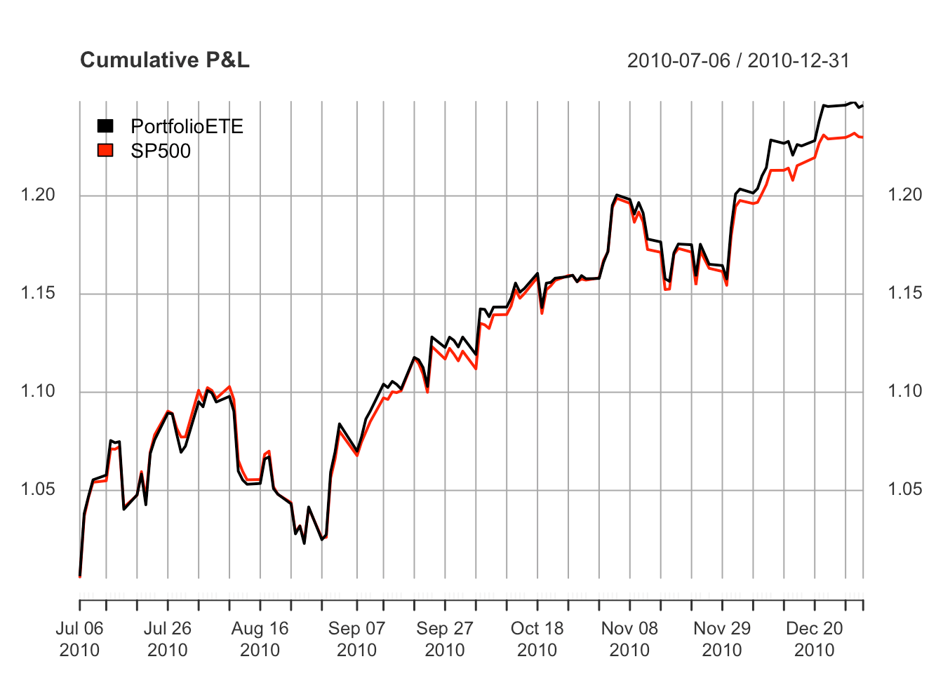
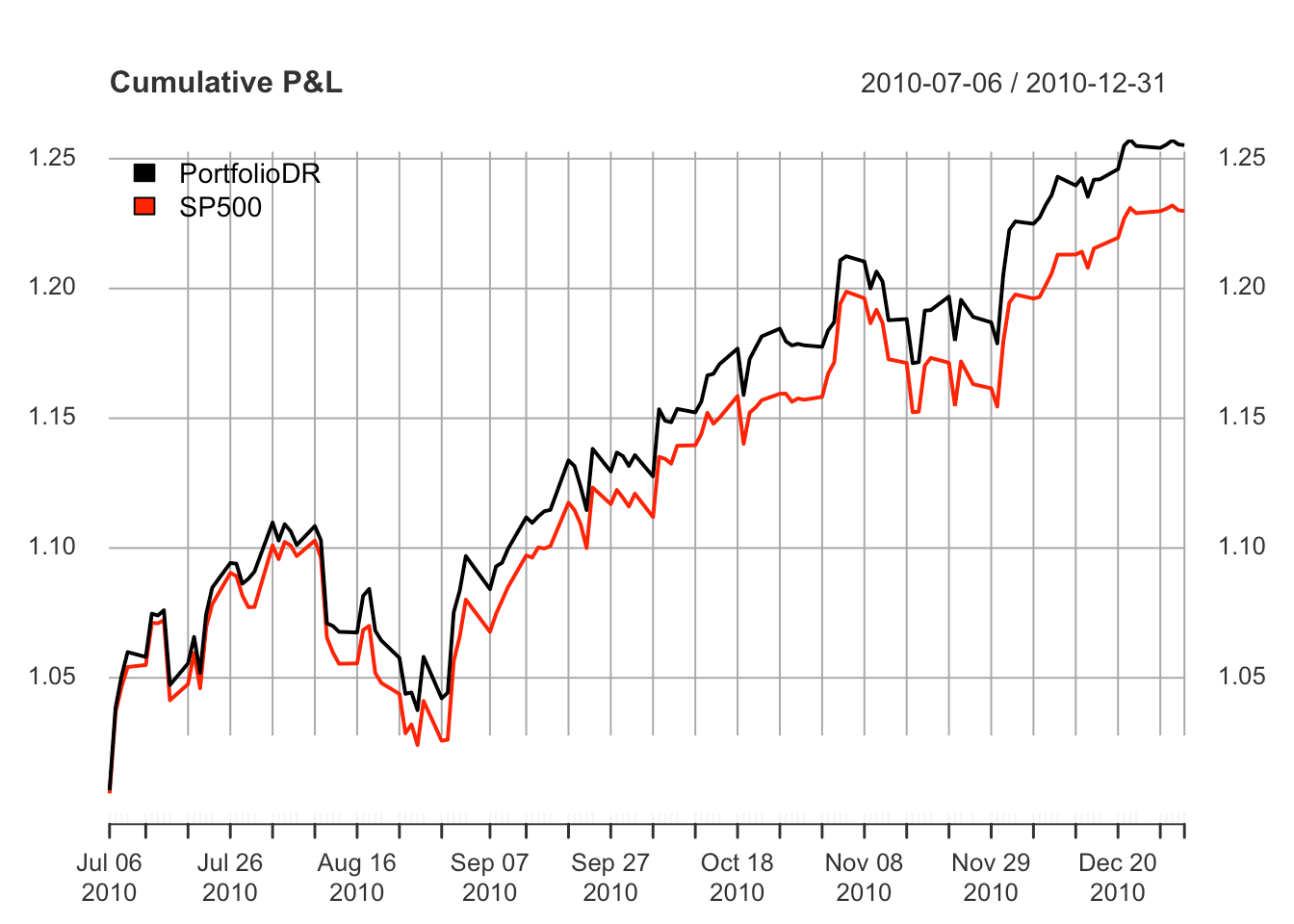
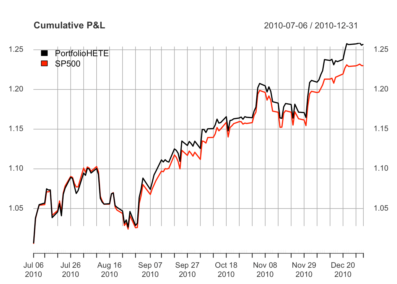
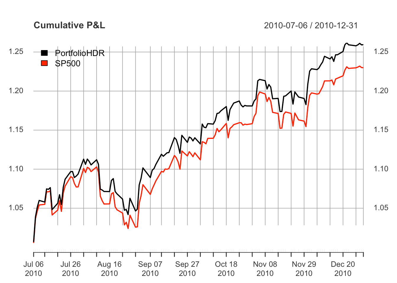
Finally, we plot the actual value of the index in the testing window in comparison with the values of the designed portfolios:
plot(cbind("PortfolioETE" = cumprod(1 + X_test %*% w_ete), cumprod(1 + r_test)),
     legend.loc = "topleft", main = "Cumulative P&L")
plot(cbind("PortfolioDR" = cumprod(1 + X_test %*% w_dr), cumprod(1 + r_test)),
     legend.loc = "topleft", main = "Cumulative P&L")
plot(cbind("PortfolioHETE" = cumprod(1 + X_test %*% w_hete), cumprod(1 + r_test)),
     legend.loc = "topleft", main = "Cumulative P&L")
plot(cbind("PortfolioHDR" = cumprod(1 + X_test %*% w_hdr), cumprod(1 + r_test)),
     legend.loc = "topleft", main = "Cumulative P&L")
README file: CRAN-readme and GitHub-readme.
Vignette: CRAN-html-vignette, CRAN-pdf-vignette, GitHub-html-vignette, and GitHub-pdf-vignette.