IRTest

IRTest can be a useful tool for IRT (item response theory) parameter estimation, especially when the violation of normality assumption on latent distribution is suspected.
IRTest deals with uni-dimensional latent variable.
In IRTest, along with the conventional approach that assumes normality on latent distribution, several methods can be applied for estimation of latent distribution:
+ empirical histogram method,
+ two-component Gaussian mixture distribution,
+ Davidian curve,
+ kernel density estimation.

Installation

You can install IRTest on R-console with:

install.packages("IRTest")

Functions

Followings are functions of IRTest available for users.

• IRTest_Dich is the estimation function when all items are dichotomously scored.

• IRTest_Poly is the estimation function when all items are polytomously scored.

• IRTest_Mix is the estimation function for a mixed-format test, a combination of dichotomous item(s) and polytomous item(s).

• DataGeneration generates several objects that are useful for computer simulation studies. Among these are starting values for an algorithm and artificial item-response data that can be passed to IRTest_Dich, IRTest_Poly, or IRTest_Mix

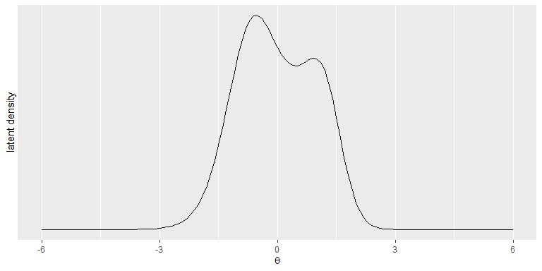
• plot_LD draws a plot of the estimated latent distribution.

• dist2 is a probability density function of two-component Gaussian mixture distribution.

• original_par_2GM converts re-parameterized parameters of two-component Gaussian mixture distribution into original parameters.

Example

A simulation study for a Rasch model can be done in following manners:

library(IRTest)

• An artificial data of 500 examinees and 10 items.

Alldata <- DataGeneration(seed = 123456789,
                          model_D = rep(1, 10),
                          N=500,
                          nitem_D = 10,
                          nitem_P = 0,
                          d = 1.664,
                          sd_ratio = 2,
                          prob = 0.3)

data <- Alldata$data_D
item <- Alldata$item_D
initialitem <- Alldata$initialitem_D
theta <- Alldata$theta

• Analysis

For an illustrative purpose, empirical histogram method is used for estimation of latent distribution.

Mod1 <- IRTest_Dich(initialitem = initialitem,
                    data = data,
                    model = rep(1, 10),
                    latent_dist = "EHM",
                    max_iter = 200,
                    threshold = .001)

• Parameter estimation results

### True item parameters 
item
#>       [,1]  [,2] [,3]
#>  [1,]    1 -0.96    0
#>  [2,]    1  0.67    0
#>  [3,]    1  0.88    0
#>  [4,]    1  0.55    0
#>  [5,]    1 -0.20    0
#>  [6,]    1  0.99    0
#>  [7,]    1  0.38    0
#>  [8,]    1  0.30    0
#>  [9,]    1  1.93    0
#> [10,]    1  0.53    0

### Estimated item parameters
Mod1$par_est
#>       a          b c
#>  [1,] 1 -0.7383615 0
#>  [2,] 1  0.5071181 0
#>  [3,] 1  0.7980726 0
#>  [4,] 1  0.5274258 0
#>  [5,] 1 -0.3909154 0
#>  [6,] 1  0.8954094 0
#>  [7,] 1  0.4264496 0
#>  [8,] 1  0.3068586 0
#>  [9,] 1  1.9525167 0
#> [10,] 1  0.4465375 0

### Plotting
par(mfrow=c(1,2))
plot(item[,2], Mod1$par_est[,2], xlab = "true", ylab = "estimated", main = "item parameters")
abline(a=0,b=1)
plot(theta, Mod1$theta, xlab = "true", ylab = "estimated", main = "ability parameters")
abline(a=0,b=1)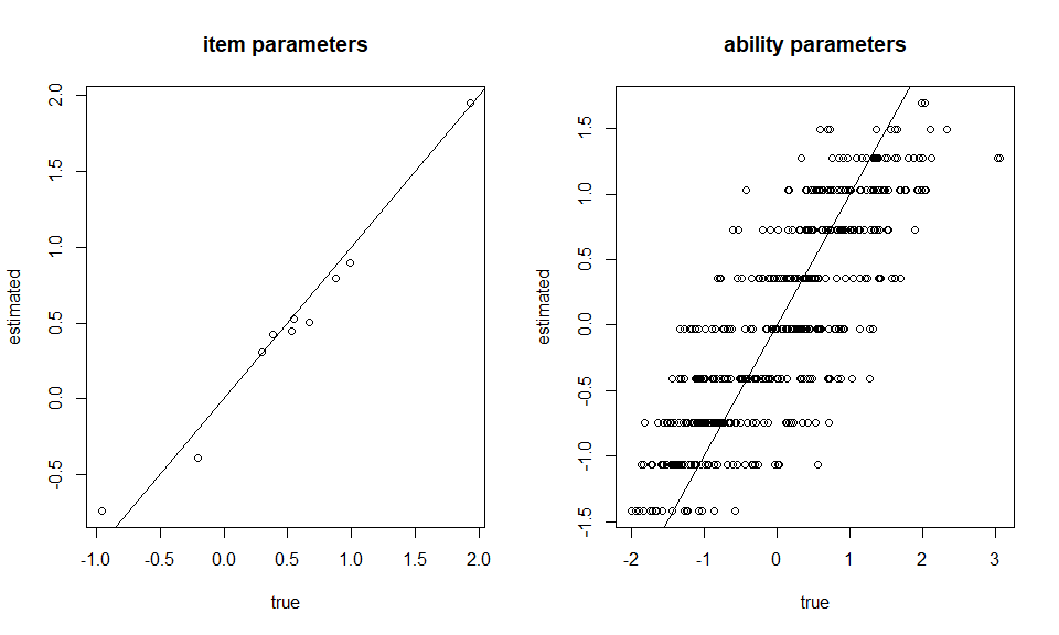

• Result of latent distribution estimation

plot_LD(Mod1)