 The above scatterplot has the following characteristics according to
scagnostics.
The above scatterplot has the following characteristics according to
scagnostics.scatteR generates scatterplots based on scagnostic measurements. The current implementation uses Simulated Annealing based on the GenSA package for optimization and rJava is required for the scagnostics measurement calculation.
Simply put scagnostics are like diagnostics for scatterplots. Each scatterplot will have a certain set of characteristics that scagnostics will show to you. You can learn more about it through this paper.
library(palmerpenguins)
library(scagnostics)
library(ggplot2)
qplot(x = bill_length_mm,y = bill_depth_mm,data=penguins)+
  theme_minimal()+
  labs(x = "Bill length",y = "Bill depth",
       title = "Scatterplot of bill length and bill depth",
       subtitle = "Data provided by palmerpenguins dataset")
The above scatterplot has the following characteristics according to
scagnostics.
scagnostics(penguins$bill_length_mm,penguins$bill_depth_mm)
#>   Outlying     Skewed     Clumpy     Sparse   Striated     Convex     Skinny
#> 0.12472358 0.74153837 0.03680493 0.04861830 0.06785714 0.56068995 0.49944162
#>    Stringy  Monotonic
#> 0.37671468 0.06405996
#> attr(,"class")
#> [1] "scagnostics"You can install the released version of scatteR from Github with:
install.packages("devtools")
devtools::install_github("janithwanni/scatteR")library(scatteR)
## basic example code
df <- scatteR(measurements = c("Monotonic" = 0.9),n_points = 100)
#> [1] "Epoch 1"
#> It: 1, obj value: 0.002060606061
#> [1] "Epoch 2"
#> It: 1, obj value: 0.002382925918
#> It: 20, obj value: 0.001763206699
#> It: 94, obj value: 0.000693521734
#> [1] "Epoch 3"
#> It: 1, obj value: 0.0009634972381
#> [1] "Epoch 4"
#> It: 1, obj value: 0.001210817323
#> [1] "Epoch 5"
#> It: 1, obj value: 0.0006452760813
#> [1] "Epoch 6"
#> It: 1, obj value: 0.0002109779468
#> [1] "Epoch 7"
#> It: 1, obj value: 4.33048594e-05
#> [1] "Epoch 8"
#> It: 1, obj value: 2.879774646e-05
#> [1] "Epoch 9"
#> It: 1, obj value: 1.78457193e-05
#> [1] "Epoch 10"
#> It: 1, obj value: 5.342541186e-05
#> [1] "Epoch 11"
#> It: 1, obj value: 0.0007308666196
#> [1] "Epoch 12"
#> It: 1, obj value: 0.003797876988
#> It: 27, obj value: 0.0001279653614
#> [1] "Epoch 13"
#> [1] "Epoch 14"
#> [1] "Epoch 15"
#> [1] "Epoch 16"
#> It: 1, obj value: 0.0001079452511
#> [1] "Epoch 17"
#> It: 1, obj value: 0.0001488984651
#> [1] "Epoch 18"
#> It: 1, obj value: 3.746684033e-05
#> [1] "Epoch 19"
#> It: 1, obj value: 4.910409006e-05
#> [1] "Epoch 20"
#> It: 1, obj value: 5.739727661e-06
#> [1] "Epoch 21"
#> It: 1, obj value: 2.171413779e-05
#> [1] "Epoch 22"
#> [1] "Epoch 23"
#> It: 1, obj value: 0.002067656372
#> It: 10, obj value: 6.65756155e-06
#> [1] "Epoch 24"
#> [1] "Epoch 25"
#> It: 1, obj value: 2.006914323e-05scagnostics(df)
#> Outlying Skewed Clumpy Sparse Striated Convex Skinny Stringy
#> 0.3374091 0.8469671 0.2213065 0.1606455 0.1296296 0.2339855 0.6467435 0.4519979
#> Monotonic
#> 0.8999799
#> attr(,"class")
#> [1] "scagnostics"plot(df$x,df$y)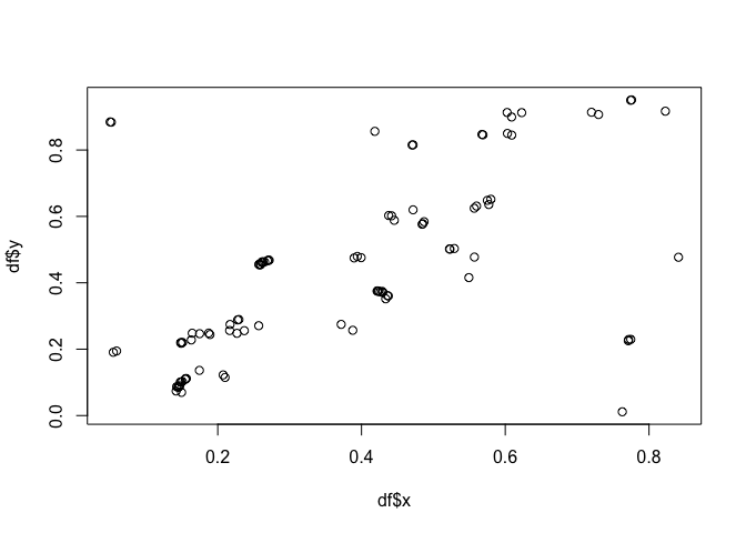
library(tidyverse)
scatteR(c("Convex" = 0.9),n_points = 250,verbose=FALSE) %>% # data generation
  mutate(label = ifelse(y > x,"Upper","Lower")) %>% # data preprocessing
  ggplot(aes(x = x,y = y,color=label))+
  geom_point()+
  theme_minimal()+
  theme(legend.position = "bottom")
generated <- scatteR(scagnostics(penguins$bill_length_mm,
                                 penguins$bill_depth_mm),
        n_points = length(penguins$bill_length_mm),verbose=FALSE)
penguins %>%
  select(bill_length_mm,bill_depth_mm) %>%
  drop_na() %>%
  rename(x = bill_length_mm,y = bill_depth_mm) %>%
  mutate(x = (x - min(x)) / (max(x) - min(x)),
         y = (y - min(y)) / (max(y) - min(y)),
         source = "penguins") %>%
  bind_rows(generated %>% mutate(source = "generated")) %>%
ggplot(aes(x = x,y = y,color=source))+
  geom_point()+
  theme_minimal()+
  theme(legend.position = "bottom")